NerveDB with data buffering

Note

Note that the data buffering feature is only available when location is set to CENTRAL when using the NerveDB as an output.

Data buffering is a feature of the NerveDB output. Its purpose is to give a guarantee that data will always reach the Management System even when a node is connected to an unstable network. When this feature is enabled, data is buffered into persistent local storage first and then sent to the Management System in chunks. New chunks are not sent until it is confirmed that the previous chunk has been stored in a database in the Management System. After the confirmation, the chunk is removed from the persistent local storage. This slows down the insert rate for very fast data sources but in exchange provides a strong guarantee that no data is lost.

This example shows how to use the data buffering feature of the NerveDB output. It uses an MQTT sensor simulation as a data source. This also requires an MQTT broker. First, the sensor simulation and the broker need to be provisioned in the Management System and deployed to the node.

Provisioning and deploying the sensor simulation and the MQTT broker

In the instructions below two Docker workloads will be provisioned and deployed:

An MQTT broker must to be deployed to the node first in order for the sensor simulation to function. The EMQX MQTT broker is used in this example that can be downloaded from the Docker Hub registry.

After that the temperature and humidity sensors simulation MQTT publisher is deployed. Download the Data Services MQTT demo sensor found under Example Applications from the Nerve Software Center. This is the Docker image that is required for provisioning the demo sensor as a Docker workload.

Log in to the Management System. Make sure that the user has the permissions to access the Data Services.

Provision a Docker workload for the EMQX MQTT broker by following Provisioning a Docker workload. This example uses emqx-4.1.0 as the workload name. Use the following workload version settings:

Setting	Value
Name	Enter any name for the workload version.
Release name	Enter any release name.
DOCKER IMAGE	Select From registry and enter `emqx/emqx:v4.1.0`.
Container name	`emqx`
Network name	`host`

Provision a Docker workload for the sensor simulation by following Provisioning a Docker workload. Use the following workload version settings:

Setting	Value
Name	Enter any name for the workload version.
Release name	Enter any release name.
DOCKER IMAGE	Select Upload to add the Docker image of the sensor simulation that has been downloaded from the Nerve Software Center.
New environment variable	Select the + icon and enter the following information: Env. variable `MQTT_PUB_TOPIC` Variable value `demo-sensor-topic`
Container name	`ttt-mqtt-demo-sensor-1.0`
Network name	`host`

Deploy both provisioned Docker workloads above by following Deploying a workload.

Configuring the Data Services Gateway

The input data is a subscription to temperature and humidity variables on the MQTT broker. The NerveDB is set as an output, with location set to CENTRAL in order for the data buffering feature to be usable. The input and output are linked in connections.

The Gateway configuration below shows that data buffering is enabled on a table level. The table demo-sensor-data has data buffering enabled with a 60 minutes expiration time. This means that if the data point is not confirmed by the Management System side in 60 minutes, it will be dropped regardless if it is written into the Management System database. Expiration time is set in minutes and in theory can be any positive value.

Follow the instructions below to apply the Gateway configuration.

Access the Local UI on the node. This is Nerve Device specific. Refer to the table below for device specific links to the Local UI. The initial login credentials to the Local UI can be found in the customer profile.

Nerve Device	Physical port	Local UI
MFN 100	P1	http://172.20.2.1:3333
Kontron KBox A-150-APL	LAN 1	`<wanip>:3333` To figure out the IP address of the WAN interface, refer to Finding out the IP address of the device in the Kontron KBox A-150-APL chapter of the device guide.
Kontron KBox A-250	ETH 2	`<wanip>:3333` To figure out the IP address of the WAN interface, refer to Finding out the IP address of the device in the Kontron KBox A-250 chapter of the device guide.
Maxtang AXWL10	LAN1	`<wanip>:3333` To figure out the IP address of the WAN interface, refer to Finding out the IP address of the device in the Maxtang AXWL10 chapter of the device guide.
Siemens SIMATIC IPC127E	X1 P1	http://172.20.2.1:3333
Siemens SIMATIC IPC427E	X1 P1	http://172.20.2.1:3333
Supermicro SuperServer E100-9AP-IA	LAN1	`<wanip>:3333` To figure out the IP address of the WAN interface, refer to Finding out the IP address of the device in the Supermicro SuperServer E100-9AP-IA chapter of the device guide.
Supermicro SuperServer 1019D-16C-FHN13TP	LAN3	http://172.20.2.1:3333
Supermicro SuperServer 5029C-T	LAN1	`<wanip>:3333` To figure out the IP address of the WAN interface, refer to Finding out the IP address of the device in the Supermicro SuperServer 5029C-T chapter of the device guide.
Toshiba FA2100T-700	First rear port	http://172.20.2.1:3333
Vecow SPC-5600-i5-8500	LAN 1	http://172.20.2.1:3333
Winmate EACIL20	LAN1	`<wanip>:3333` To figure out the IP address of the WAN interface, refer to Finding out the IP address of the device in the Winmate EACIL20 chapter of the device guide.

Select the arrow next to Data to expand the Data Services sub menus in the navigation on the left.
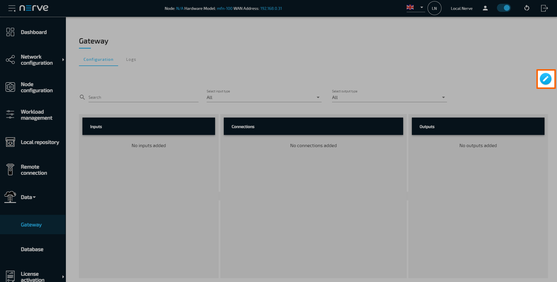
Select Gateway.
Select the Edit configuration icon on the right to enter editing mode.

Create a JSON file out of the following Gateway configuration:

{
    "inputs": [
        {
            "type": "MQTT_SUBSCRIBER",
            "clientId": "mqtt_sub_dbuf-in",
            "serverUrl": "tcp://localhost:1883",
            "keepAliveInterval_s": 20,
            "cleanSession": true,
            "qos": 1,
            "connectors": [
                {
                    "topic": "demo-sensor-topic",
                    "variables": [
                        {
                            "name": "temperature",
                            "type": "int16"
                        },
                        {
                            "name": "humidity",
                            "type": "uint16"
                        }
                    ]
                }
            ]
        }
    ],
    "outputs": [
        {
            "type": "NERVE_DB",
            "location": "CENTRAL",
            "connectors": [
                {
                    "tableName": "demo-sensor-data",
                    "dataBuffer": true,
                    "bufferExpTime": 60
                }
            ]
        }
    ],
    "connections" : [
        {
            "input": { "index" : 0, "connector" : 0 },
            "output": { "index" : 0, "connector" : 0 }
        }
    ]
}

Select the Import button.
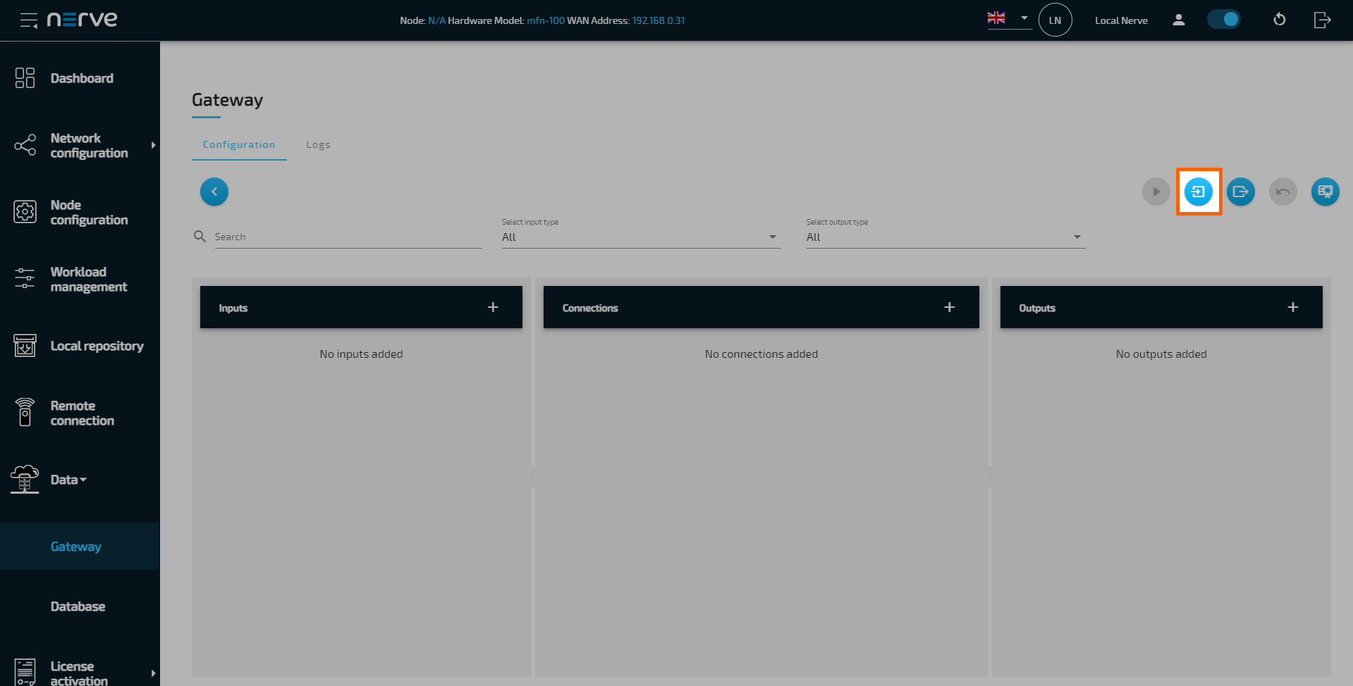
Add the JSON configuration file containing the code above from the file browser.
Select the Deploy button. A success message pops up in the upper-right corner.

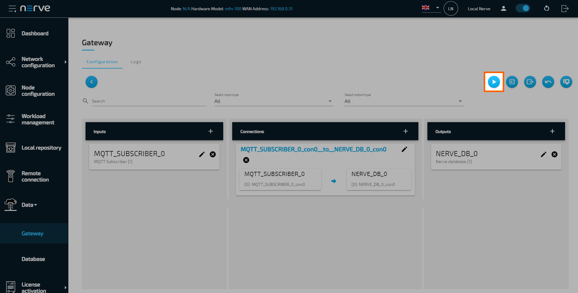
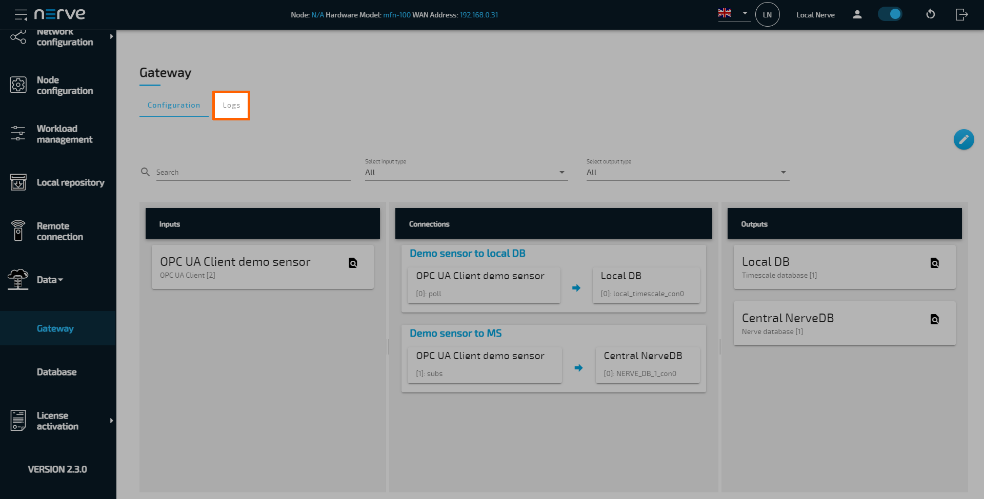
The configuration is now deployed. The graphical configuration tool now reflects the contents of the JSON file. Exit editing mode by selecting the arrow on the left. Details of each input and output can be opened by selecting the magnifying glass symbol next to each input and output.

Select the Logs tab to view the Gateway logs for more information.

To test whether data buffering is working as intended a faulty network can be simulated, for example by unplugging the network cable of the device. Since the data source is deployed as a workload, it will not be affected by an outside connection and the data should keep flowing. Once the connection has been restored, depending on the amount of data that is buffered on the device it should reach the Management System in due time. This process can be repeated multiple times.

Central data visualization in the Management System

The arrival of data may be monitored in real time using Grafana. To visualize the data received by the Gateway, open the cental data visualization element through the Data Services UI in the Management System.

Select Data in the navigation on the left. The Grafana UI will open.

Note

Note that the navigation on the left collapses when Data is selected. Select the burger menu in the top-left to expand the navigation again.
Select + > Dashboard in the navigation on the left. A box will appear.
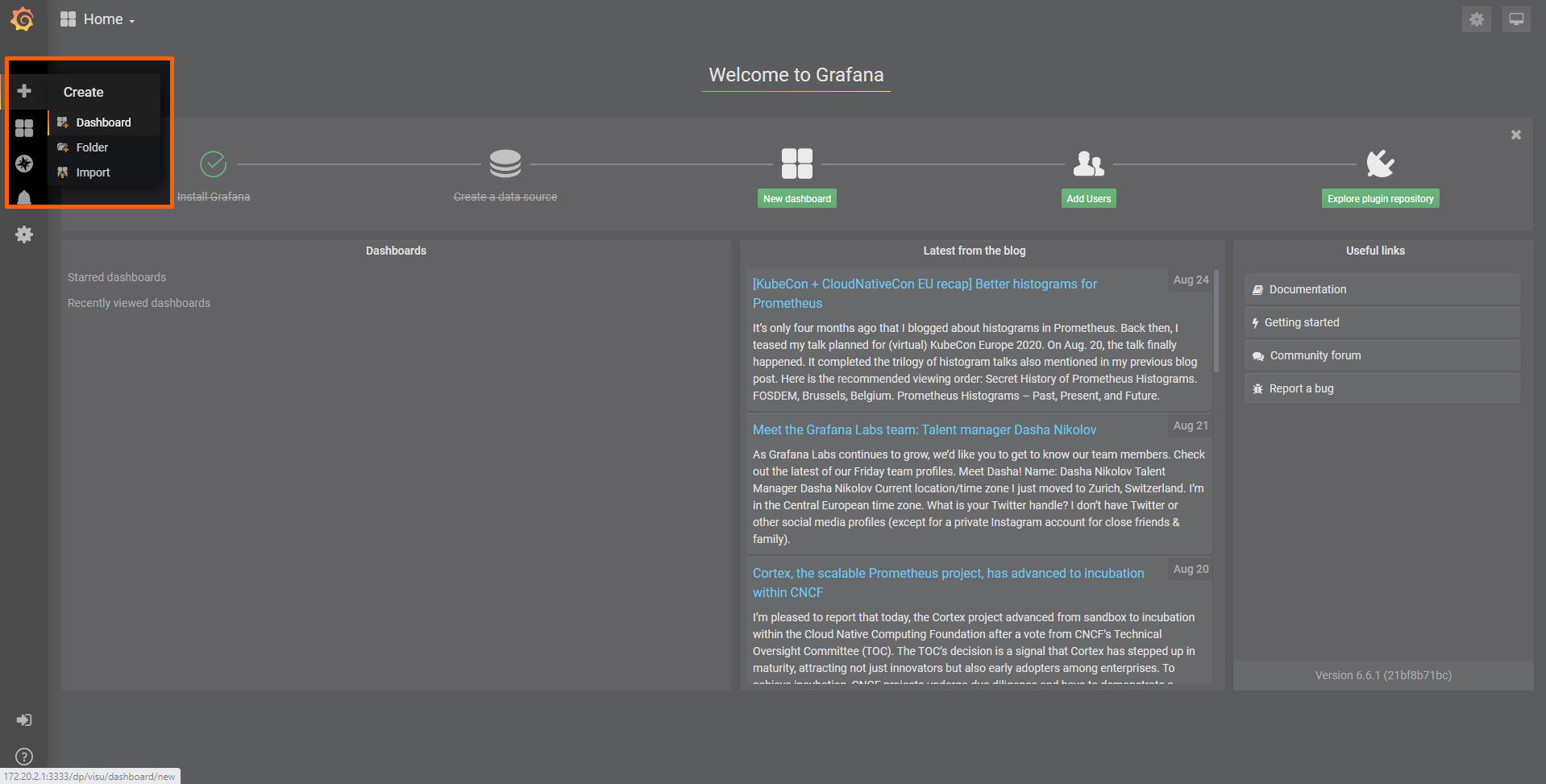
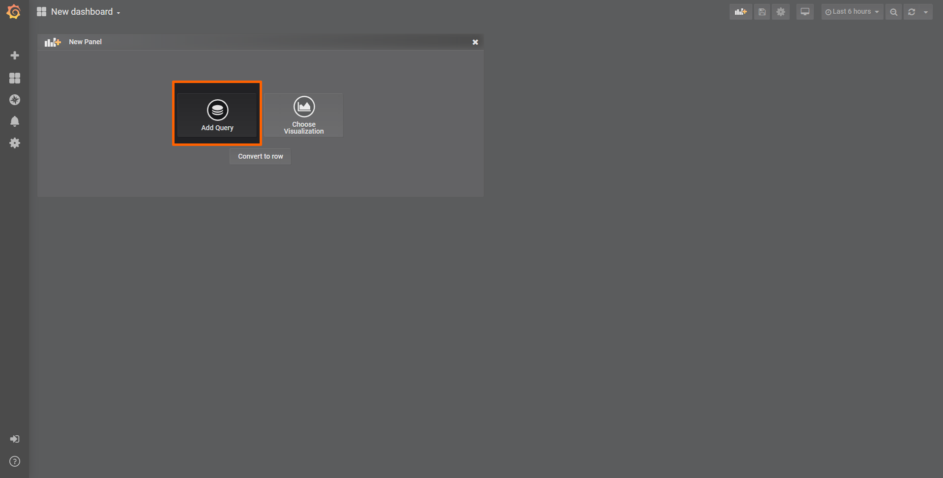
Select Add Query in the New Panel box.
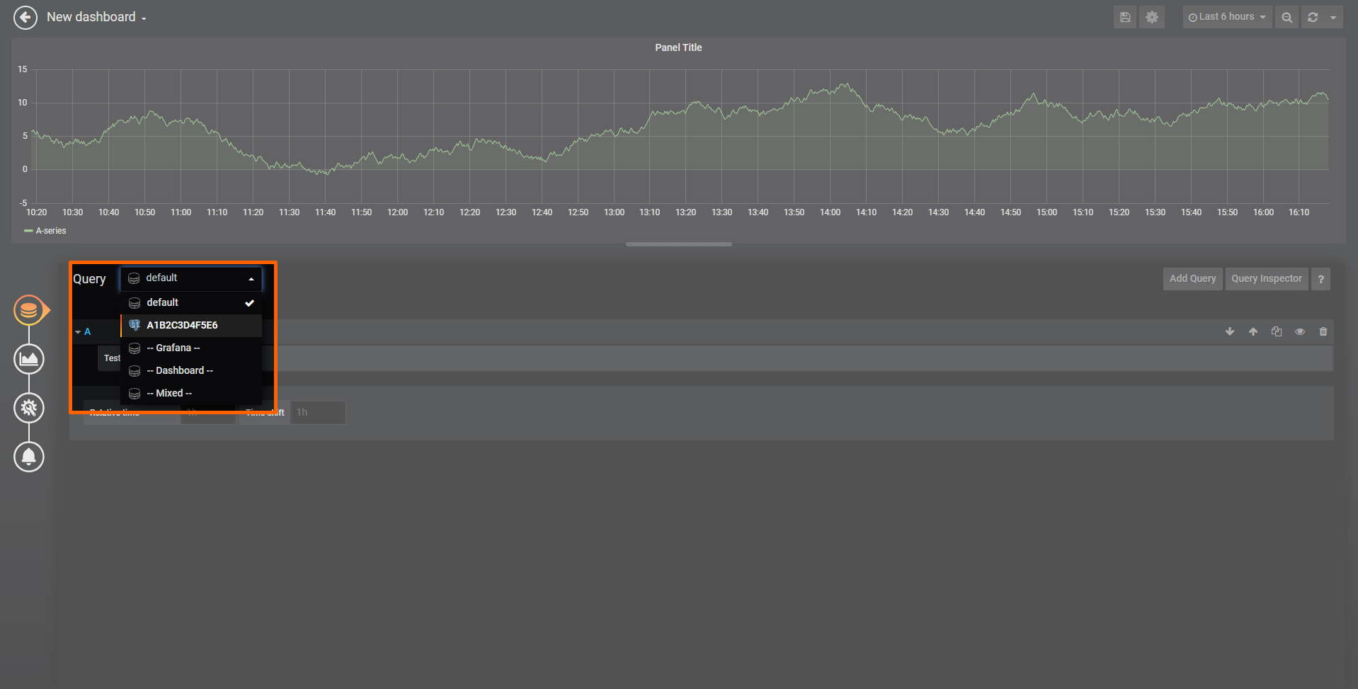
Select the data source from the drop-down menu. The name of the data source is the serial number of the node.
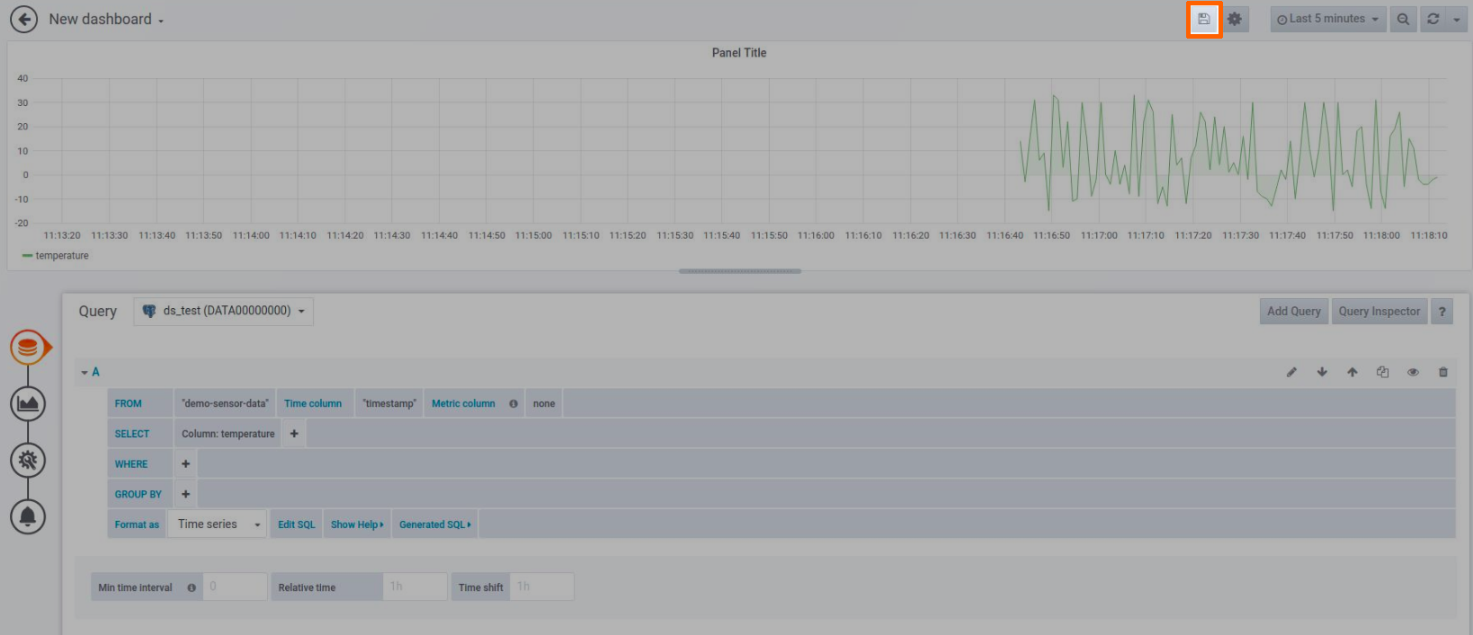
Fill in the following query information to add the temperature data from the MQTT Subscriber:

Setting Value

FROM mqttsub_timescaledb_0

Time column: "timestamp"

SELECT Column: temperature

Format as Time series
Select the save icon in the upper-right corner to save the dashboard.

The dashboard can be accessed from the Grafana home menu.

Setting	Value
FROM	`mqttsub_timescaledb_0` Time column: "timestamp"
SELECT	Column: temperature
Format as	Time series