Custom JSON format example
Note
This example is partially deprecated and needs to be updated. The variable expansion operator [*] has been dropped in favor of the native array support available on all JSON inputs and outputs.
In this example, data is provided to the Nerve Data Services Gateway in a custom JSON format. Compared to the previous version of the Gateway, data can be input more freely, as it was previously required to strictly adhere to the JSON format of the Gateway.
The data in the custom JSON format is provided by an MQTT Publisher in form of a demo sensor to be processed and stored by the Gateway for visualization at the node.
Provisioning and deploying the sensor simulation and the MQTT broker
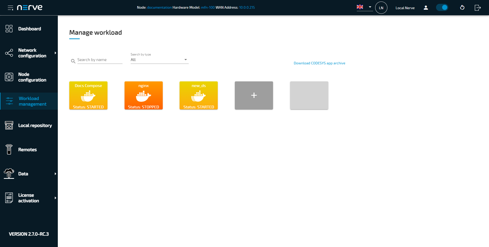
In the instructions below two Docker workloads will be provisioned and deployed:
An MQTT broker must to be deployed to the node first in order for the sensor simulation to function. The EMQX MQTT broker is used in this example that can be downloaded from the Docker Hub registry.
Afterwards the temperature and humidity sensors simulation MQTT publisher is deployed. Download the Data Services MQTT demo sensor found under Example Applications from the Nerve Software Center. This is the Docker image that is required for provisioning the demo sensor as a Docker workload.
- Log in to the Management System. Make sure that the user has the permissions to access the Data Services.
-
Provision a Docker workload for the EMQX MQTT broker by following Provisioning a Docker workload. This example uses emqx-4.1.0 as the workload name. Use the following workload version settings:
Setting Value Name Enter any name for the workload version. Release name Enter any release name. DOCKER IMAGE Select From registry and enter emqx/emqx:v4.1.0.Container name emqxNetwork name host -
Provision a Docker workload for the sensor simulation by following Provisioning a Docker workload. Use the following workload version settings:
Setting Value Name Enter any name for the workload version. Release name Enter any release name. DOCKER IMAGE Select Upload to add the Docker image of the sensor simulation that has been downloaded from the Nerve Software Center. New environment variable Select the + icon and enter the following information: - Env. variable
MQTT_PUB_TOPIC - Variable value
demo-sensor-topic
Container name ttt-mqtt-demo-sensor-1.0Network name host - Env. variable
-
Deploy both provisioned Docker workloads above by following Deploying a workload.
Configuring the Data Services Gateway
The Gateway configuration in the instructions below defines an MQTT subscriber as an input that receives data in a custom JSON format on four different topics. The output is a TimescaleDB database with four different tables, one per topic.
-
Access the Local UI on the node. This is Nerve Device specific. Refer to the table below for device specific links to the Local UI. The initial login credentials to the Local UI can be found in the customer profile.
Nerve Device Physical port Local UI MFN 200 P3 http://172.20.2.1:3333 MFN 100 P1 http://172.20.2.1:3333 Kontron KBox A-250 ETH 2 <wanip>:3333
To figure out the IP address of the WAN interface, refer to Finding out the IP address of the device in the Kontron KBox A-250 chapter of the device guide.Siemens SIMATIC IPC427E X1 P1 http://172.20.2.1:3333 Siemens SIMATIC IPC BX-39A X1 P1 http://172.20.2.1:3333 Vecow SPC-5600-i5-8500 LAN 1 http://172.20.2.1:3333 Compulab fitlet3 LAN3 http://172.20.2.1:3333 -
Select the arrow next to Data to expand the Data Services sub menus in the navigation on the left.
- Select Gateway.
-
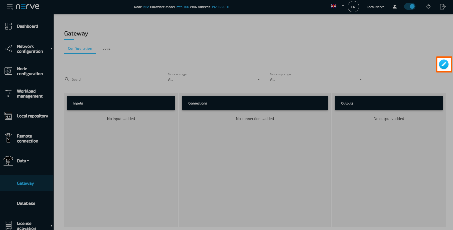
Select the Edit configuration icon on the right to enter editing mode.
-
Create a JSON file out of the following Gateway configuration:
{ "inputs": [ { "type": "MQTT_SUBSCRIBER", "name": "mqtt_subscriber", "clientId": "mqtt_subscriber_0", "serverUrl": "tcp://localhost:1883", "keepAliveInterval_s": 20, "cleanSession": true, "qos": 1, "connectors": [ { "name": "mqtt_subscriber_connector_0", "topic": "machineA", "variables": [ { "name": "temperature", "type": "int32", "path": ".machineA.temperatureSensor" }, { "name": "top-left.distance", "type": "double", "path": ".machineA.distance_sensors" }, { "name": "top-right.distance", "type": "double", "path": ".machineA.distance_sensors" }, { "name": "bottom-left.distance", "type": "double", "path": ".machineA.distance_sensors" }, { "name": "bottom-right.distance", "type": "double", "path": ".machineA.distance_sensors" } ] }, { "name": "mqtt_subscriber_connector_1", "topic": "machineB", "timestamp": { "path": ".info.measurement_time[]" }, "variables": [ { "type": "int32", "path": ".machineB.sensor1[].temperature" }, { "type": "uint32", "path": ".machineB.sensor1[].humidity" }, { "type": "int32", "path": ".machineB.sensor2[].temperature" }, { "type": "uint32", "path": ".machineB.sensor2[].humidity" } ] }, { "name": "mqtt_subscriber_connector_2", "topic": "machineC", "variables": [ { "type": "string", "path": ".machineC[*].entry", "maxValues": 4 } ] }, { "name": "mqtt_subscriber_connector_3", "topic": "all_combined", "variables": [ { "type": "uint8", "path": "[*].[]", "maxValues": 11 }, { "type": "uint8", "path": "[].[*]", "maxValues": 11 } ] } ] } ], "outputs": [ { "type":"DB_TIMESCALE", "name":"outp_timescale", "url":"<LOCAL>", "connectors": [ { "tableName": "machineA_data" }, { "tableName": "machineB_data" }, { "tableName": "machineC_data" }, { "tableName": "all_combined_data" } ] } ], "connections": [ { "name": "connection_0", "input": { "index": 0, "connector": 0 }, "output": { "index": 0, "connector": 0 } }, { "name": "connection_1", "input": { "index": 0, "connector": 1 }, "output": { "index": 0, "connector": 1 } }, { "name": "connection_2", "input": { "index": 0, "connector": 2 }, "output": { "index": 0, "connector": 2 } }, { "name": "connection_3", "input": { "index": 0, "connector": 3 }, "output": { "index": 0, "connector": 3 } } ] } -
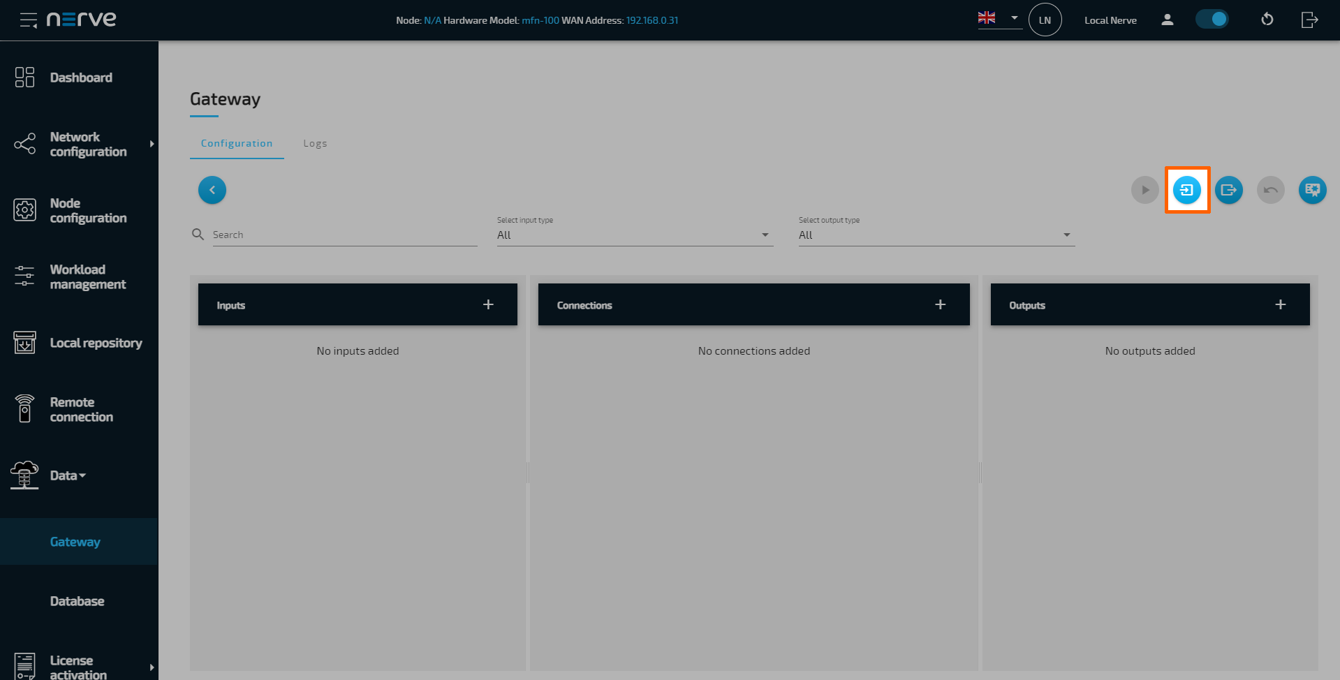
Select the Import button.
-
Add the JSON configuration file containing the code above from the file browser.
-
Select the Deploy button. A success message pops up in the upper-right corner.
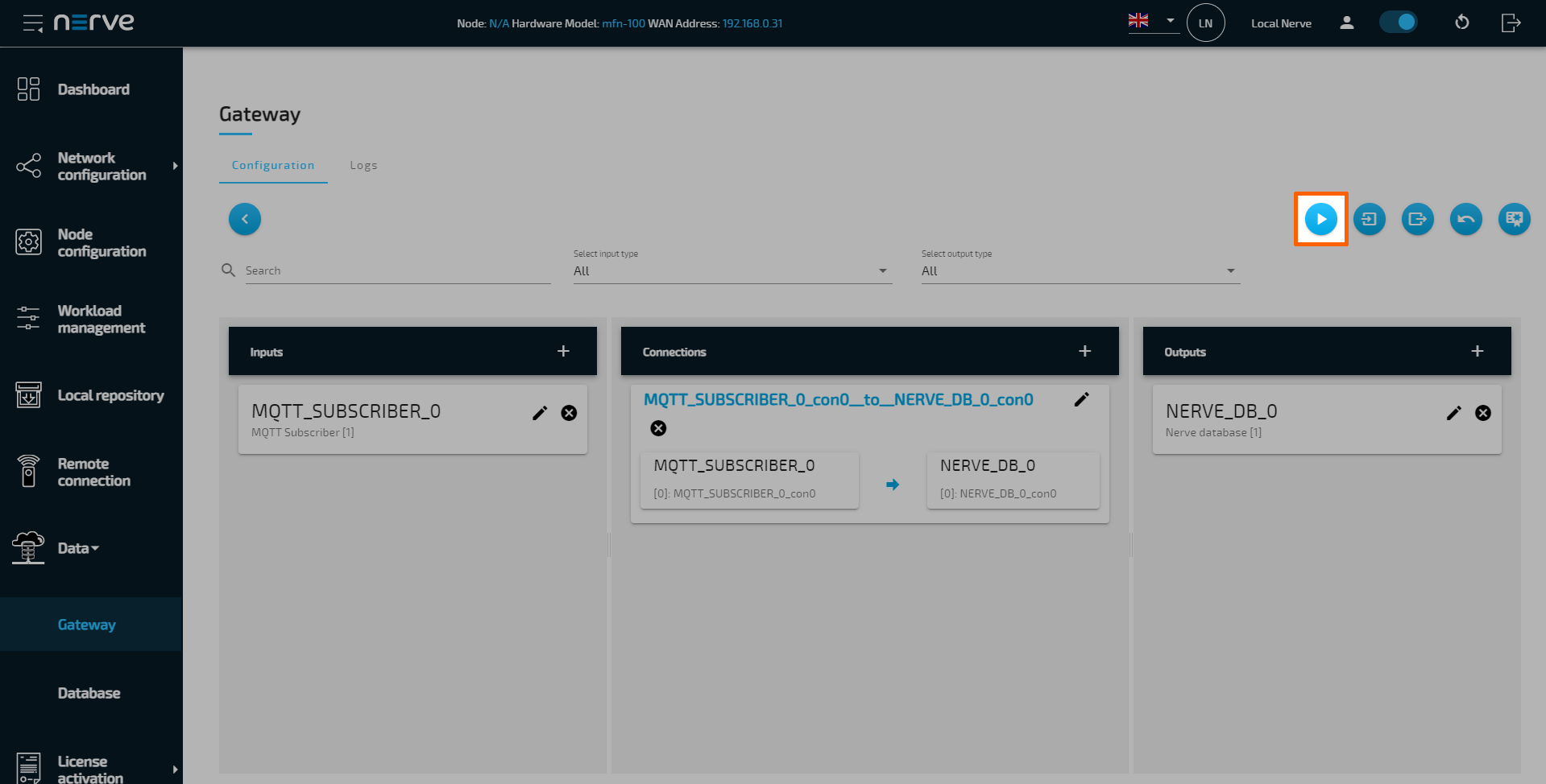
The configuration is now deployed. The graphical configuration tool now reflects the contents of the JSON file. Exit editing mode by selecting the arrow on the left. Details of each input and output can be opened by selecting the magnifying glass symbol next to each input and output.
Select the Logs tab to view the Gateway logs for more information.
Taking a closer look at the data
The input is an MQTT Subscriber that receives data in custom JSON format on four different topics. The output is a TimescaleDB database with four different tables, one per topic or data.
First connector data
The first connector receives data from a simulation sensor:
{
    "machineA": {
        "type": "molding",
        "date_installed": "2018-07-03",
        "temperatureSensor": {
            "state": "MEASURING",
            "hasError": false,
            "temperature": 34
        },
        "distance_sensors": {
            "top-left": {
                "distance": 0.26210331244354845,
                "hasError": false
            },
            "top-right": {
                "distance": 0.26046464329587893,
                "hasError": false
            },
            "bottom-left": {
                "distance": 0.6323130733349438,
                "hasError": false
            },
            "bottom-right": {
                "distance": 0.8431831637166814,
                "hasError": false
            }
        }
    }
}
With the configuration above only data that is defined in the Gateway configuration is extracted and written into the database. By specifying exactly which fields value is required, all other data is eliminated. This gives flexibility to the Gateway to support all kinds of JSON formats.
Example data table
| top‑left.distance | top‑right.distance | bottom‑left.distance | bottom‑right.distance | temperature |
|---|---|---|---|---|
| 0.26210331244354845 | 0.26046464329587893 | 0.6323130733349438 | 0.8431831637166814 | 34 |
Second connector data
The second connector also receives data from a simulation server, but in batches:
{
    "info": {
        "measurement_time": [
            1611936105084752100,
            1611936105084770000,
            1611936105084773000
        ]
    },
    "machineB": {
        "sensor1": [
            {
                "temperature": 25,
                "humidity": 24
            },
            {
                "temperature": 26,
                "humidity": 100
            },
            {
                "temperature": 28,
                "humidity": 78
            }
        ],
        "sensor2": [
            {
                "temperature": -11,
                "humidity": 84
            },
            {
                "temperature": 33,
                "humidity": 5
            },
            {
                "temperature": -11,
                "humidity": 88
            }
        ]
    }
}
With the configuration for this connector, the Gateway extracts lists of data. For example, the sensor1[].temperature list expansion extracts all temperature field values from sensor1. Note that the sensor1 array must have objects with the same fields. This also applies to sensor1[].humidity, sensor2[].temperature and sensor2[].humidity. Combining all list expansions for the data example above, the Gateway inserts three rows in the database. Each row is constructed by the field index in the JSON.
Example data table
| .machineB.sensor1[].temperature | .machineB.sensor1[].humidity | .machineB.sensor2[].temperature | .machineB.sensor2[].humidity |
|---|---|---|---|
| 25 | 24 | -11 | 84 |
| 26 | 100 | 33 | 5 |
| 28 | 78 | -11 | 88 |
Third connector data
The third connector also receives data in batches:
{
    "machineC": [
        {
            "entry": "mywclgbwcl"
        },
        {
            "entry": "ctuswukfqp"
        },
        {
            "entry": "maaqnyssvq"
        },
        {
            "entry": "usepjkpylg"
        }
    ]
}
Here only a single array of data is received to show the use of the variable expansion. The Gateway reads machineC[*].entry as a list of entries. However, instead of inserting four rows into the database, it inserts one row with four columns. Each column is labelled with the name of the values field and extended with an index of the field in the array. By supporting variable expansion, the Gateway can fetch multiple variables from a JSON without specifying them all.
Example data table
| .machineC[*].entry‑0 | .machineC[*].entry‑1 | .machineC[*].entry‑2 | .machineC[*].entry‑3 |
|---|---|---|---|
| mywclgbwcl | ctuswukfqp | maaqnyssvq | usepjkpylg |
Fourth connector data
The last connector shows the use case of combining list and variable expansions in a single Gateway variable:
[
    [0, 1, 2, 3, 4, 5, 6, 7, 8, 9, 10],
    [0, 1, 2, 3, 4, 5, 6, 7, 8, 9, 10],
    [0, 1, 2, 3, 4, 5, 6, 7, 8, 9, 10],
    [0, 1, 2, 3, 4, 5, 6, 7, 8, 9, 10],
    [0, 1, 2, 3, 4, 5, 6, 7, 8, 9, 10],
    [0, 1, 2, 3, 4, 5, 6, 7, 8, 9, 10],
    [0, 1, 2, 3, 4, 5, 6, 7, 8, 9, 10],
    [0, 1, 2, 3, 4, 5, 6, 7, 8, 9, 10],
    [0, 1, 2, 3, 4, 5, 6, 7, 8, 9, 10],
    [0, 1, 2, 3, 4, 5, 6, 7, 8, 9, 10],
    [0, 1, 2, 3, 4, 5, 6, 7, 8, 9, 10]
]
The first variable specifies the variable expansion first and the list expansion second ([*].[]). This means that a variable is each individual array and that array values are fetched as a list. Ten columns are created with ten rows inserted. Each row holds its respective value (first row, all 0, second row, all 1...).
| [*].[]-0 | [*].[]-1 | [*].[]-2 | [*].[]-3 | [*].[]-4 | [*].[]-5 | [*].[]-6 | [*].[]-7 | [*].[]-8 | [*].[]-9 | [*].[]-10 |
|---|---|---|---|---|---|---|---|---|---|---|
| 0 | 0 | 0 | 0 | 0 | 0 | 0 | 0 | 0 | 0 | |
| 1 | 1 | 1 | 1 | 1 | 1 | 1 | 1 | 1 | 1 | |
| 2 | 2 | 2 | 2 | 2 | 2 | 2 | 2 | 2 | 2 | |
| 3 | 3 | 3 | 3 | 3 | 3 | 3 | 3 | 3 | 3 | |
| 4 | 4 | 4 | 4 | 4 | 4 | 4 | 4 | 4 | 4 | |
| 5 | 5 | 5 | 5 | 5 | 5 | 5 | 5 | 5 | 5 | |
| 6 | 6 | 6 | 6 | 6 | 6 | 6 | 6 | 6 | 6 | |
| 7 | 7 | 7 | 7 | 7 | 7 | 7 | 7 | 7 | 7 | |
| 8 | 8 | 8 | 8 | 8 | 8 | 8 | 8 | 8 | 8 | |
| 9 | 9 | 9 | 9 | 9 | 9 | 9 | 9 | 9 | 9 | |
| 10 | 10 | 10 | 10 | 10 | 10 | 10 | 10 | 10 | 10 |
The second variable specifies the list expansion first and the variables expansion second ([].[*]). This means that a variable is a single element in an array and that values are fetched from all arrays for that element. Ten columns are created with ten rows inserted. Each column holds its respective value (first column, all 0, second column, all 1...).
| [].[*]-0 | [].[*]-1 | [].[*]-2 | [].[*]-3 | [].[*]-4 | [].[*]-5 | [].[*]-6 | [].[*]-7 | [].[*]-8 | [].[*]-9 | [].[*]10 |
|---|---|---|---|---|---|---|---|---|---|---|
| 0 | 1 | 2 | 3 | 4 | 5 | 6 | 7 | 8 | 9 | 10 |
| 0 | 1 | 2 | 3 | 4 | 5 | 6 | 7 | 8 | 9 | 10 |
| 0 | 1 | 2 | 3 | 4 | 5 | 6 | 7 | 8 | 9 | 10 |
| 0 | 1 | 2 | 3 | 4 | 5 | 6 | 7 | 8 | 9 | 10 |
| 0 | 1 | 2 | 3 | 4 | 5 | 6 | 7 | 8 | 9 | 10 |
| 0 | 1 | 2 | 3 | 4 | 5 | 6 | 7 | 8 | 9 | 10 |
| 0 | 1 | 2 | 3 | 4 | 5 | 6 | 7 | 8 | 9 | 10 |
| 0 | 1 | 2 | 3 | 4 | 5 | 6 | 7 | 8 | 9 | 10 |
| 0 | 1 | 2 | 3 | 4 | 5 | 6 | 7 | 8 | 9 | 10 |
| 0 | 1 | 2 | 3 | 4 | 5 | 6 | 7 | 8 | 9 | 10 |
Local data visualization at the node
To visualize the data received by the Gateway, open the local data visualization element through the Data Services UI on the node. Two separate queries will be added in the instructions below.
Visualizing machineA data
-
Select Data in the navigation on the left. The Grafana UI will open.
Note
Note that the navigation on the left collapses when Data is selected. Select the burger menu in the top-left to expand the navigation again.
-
Select + > Dashboard in the navigation on the left. A box will appear.
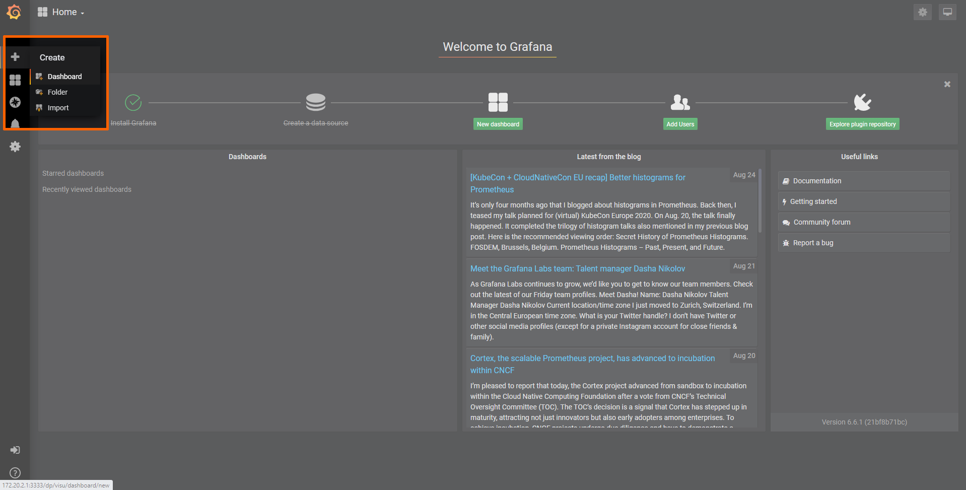
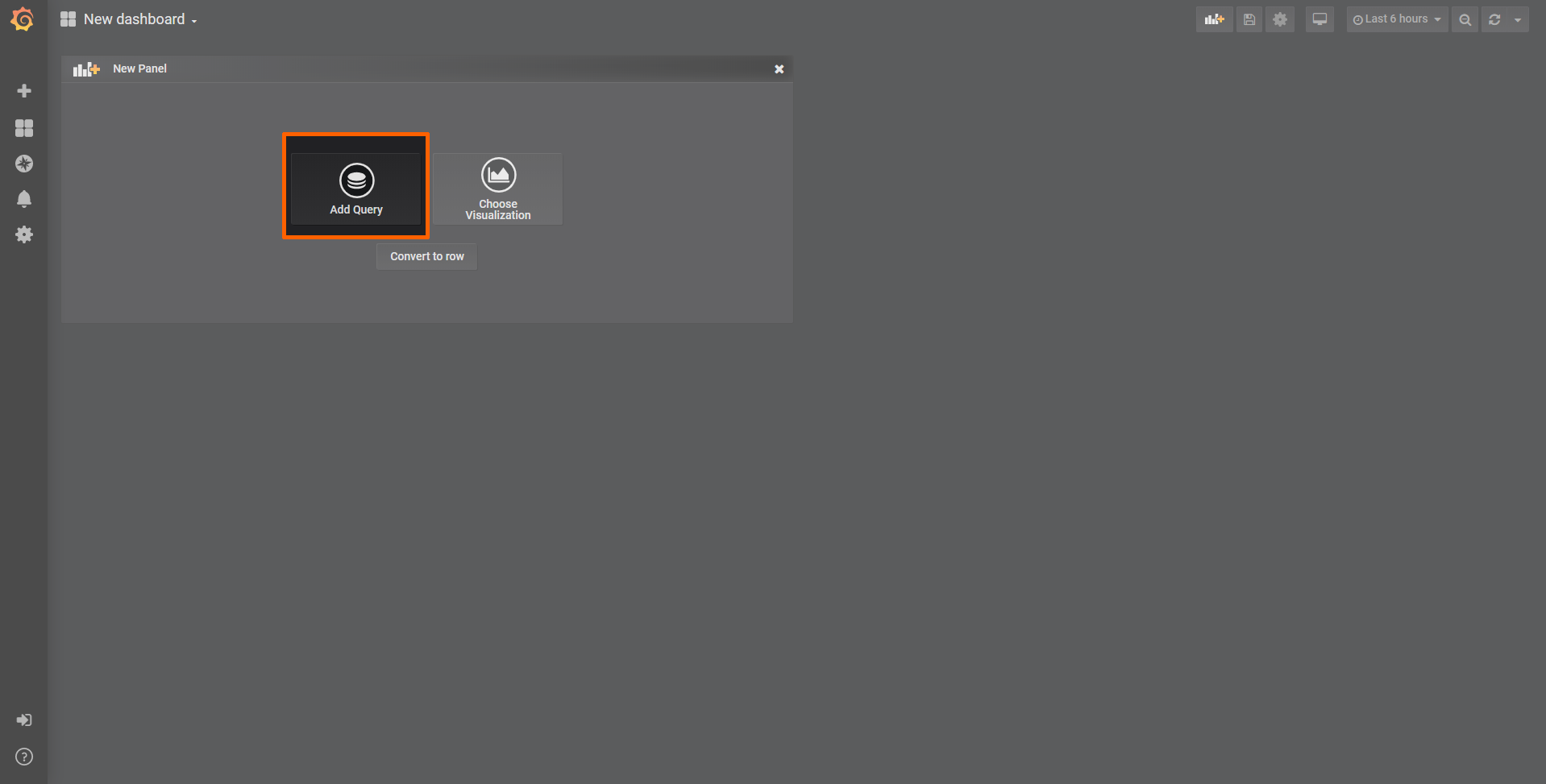
-
Select Add Query in the New Panel box.
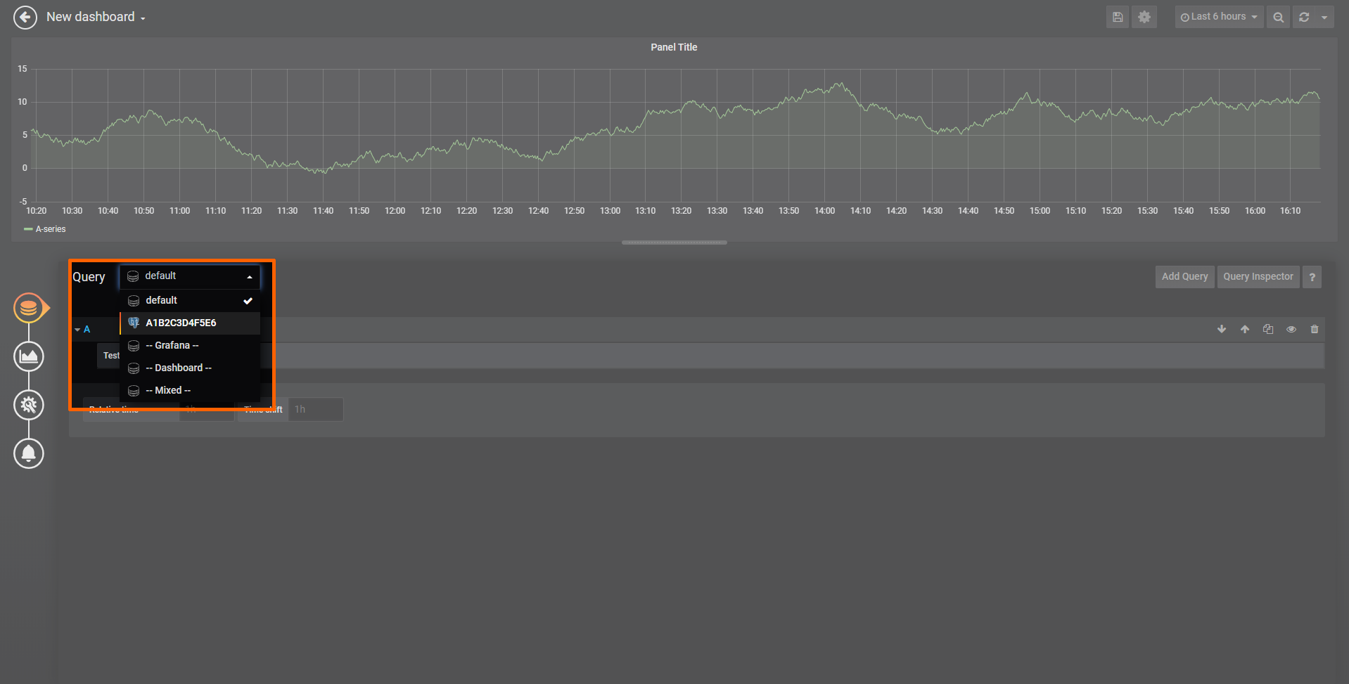
-
Select the data source from the drop-down menu. The name of the data source is the serial number of the node.
-
Fill in the following query information to add the data of Machine A:
Setting Value FROM machineA_data
Time column: "timestamp"SELECT Column: "bottom-left.distance"
Column: "bottom-right.distance"
Column: "top-left.distance"
Column: "top-right.distance"Format as Time series -
Select the save icon in the upper-right corner to save the dashboard.
The dashboard can be accessed from the Grafana home menu.
Visualizing machineB data
-
Select Data in the navigation on the left. The Grafana UI will open.
Note
Note that the navigation on the left collapses when Data is selected. Select the burger menu in the top-left to expand the navigation again.
-
Select + > Dashboard in the navigation on the left. A box will appear.
-
Select Add Query in the New Panel box.
-
Select the data source from the drop-down menu. The name of the data source is the serial number of the node.
-
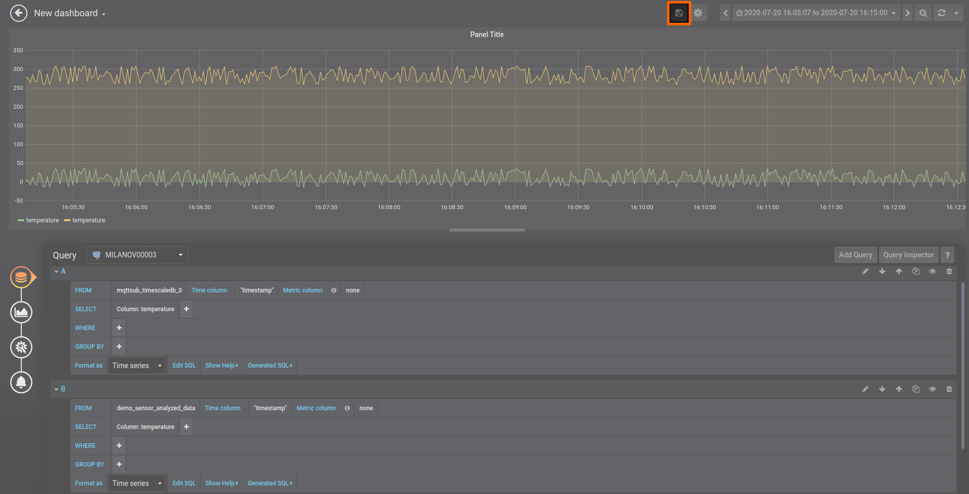
Fill in the following query information to add the data of Machine B:
Setting Value FROM machineB_data
Time column: "timestamp"SELECT Column: ".machineB.sensor1[].humidity"
Column: ".machineB.sensor1[].temperature"
Column: ".machineB.sensor2[].humidity"
Column: ".machineB.sensor2[].temperature"Format as Time series -
Select the save icon in the upper-right corner to save the dashboard.
The dashboard can be accessed from the Grafana home menu.