Tutorial: Real-time performance monitoring
Nerve is a platform to run applications in form of Docker containers and virtual machines on edge computers. It also contains a PLC runtime, executed as a virtual machine on the device. This tutorial shows how to measure the real-time performance of an IEC 61131-3 PLC application and therefore provides insight on the performance of the ACRN hypervisor and Intel TCC technologies supported by Intel’s Edge Controls for Industrial (ECI) included in Nerve. It will also show you how to manage software at the edge using Nerve and how to use the remote access features as well as the monitoring features of Nerve.
Going through this demo will take about 30 minutes and cover how to deploy container workloads, remotely access nodes, configure the Nerve Data Services and view data in an integrated version of Grafana in the Nerve Data Services.
Items needed for this tutorial are:
- a workstation or PC
- login credentials to the Nerve Management System and the filesharing server
- the Nerve Connection Manager app
- a Gateway configuration file
- a Grafana dashboard configuration file
All links, login credentials and the instructions to download files will be sent via emails. In case files or login credentials are missing, contact trynerve@tttech-industrial.com.
The tutorial environment is set up in the evaluation laboratory at TTTech Industrial in Vienna. The edge device is an MFN 100 or a Maxtang AXWL10 running an Intel Atom quad core CPU.
Note
In case the evaluation system is used, be aware that other users may access the same evaluation system, meaning that other nodes might be registered in the Management System. Information and workloads uploaded into the system may be visible to other users.
Architecture of the Edge Device
The consistent real-time performance of a PLC independent of all other influences on the same device is most important for controls or high-speed data acquisition. Nerve enables users to install many different types of applications on the same devices as the soft PLC. Therefore, it is important that those applications – Docker containers or virtual machines – do not influence real-time performance. Intel’s TCC features and the ACRN hypervisor build the basis for the necessary performance and separation.
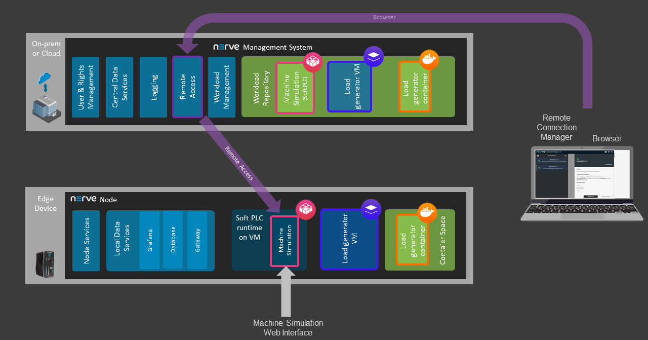
The graphic below shows the main components of a Nerve based edge device, which we call Nerve Device. The highlighted components are the relevant ones for this tutorial.
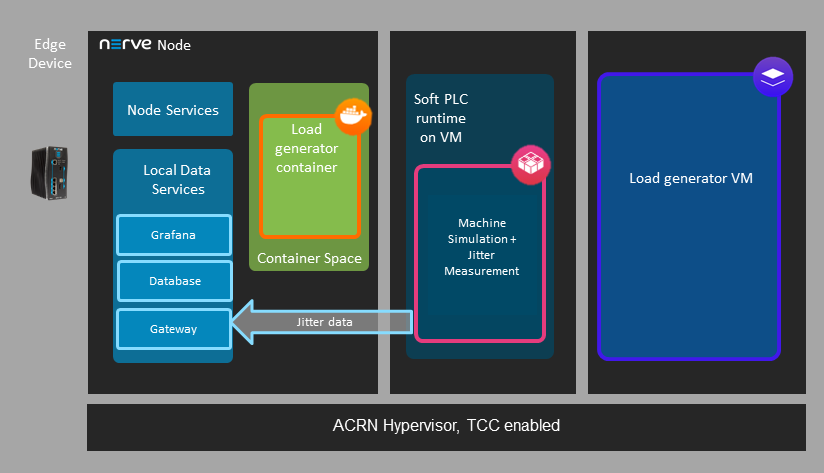
Machine Simulation
The machine simulation is a small program written in IEC-61131-3. It simulates the operation of a CNC mill and generates data in the process. The simulated machine as such is not of interest for this tutorial. Instead, the tutorial focuses on the real-time performance of the PLC application running this simulation. Besides creating the simulation data, the PLC application also measures and provides its internal task latencies and jitter values to proof performance and isolation achieved through virtualization. The measured simulation, latency and jitter data is provided through the integrated OPC UA server.
Load Generator applications
A VM and a Docker container are prepared as workloads to generate a load on the system. The small virtual machine is configured to take two CPU cores and load them heavily. It also tries to force cache flushes as much as possible to load the CPU and maximize interference with other CPU cores. The Docker container also loads the CPU heavily in terms of RAM consumption and calculation.
Gateway
The Gateway application is a multiprotocol translator integrated in Nerve which can read data from various sources and provide it with high performance to other systems like MQTT brokers, databases, Kafka or the Azure IoT Hub. In this tutorial it is used to read jitter and latency data from the OPC UA server and feed it to the Nerve integrated database.
Database
The integrated database is designed to receive data from the Gateway for further analytics. It can be used by any application on Nerve as a general time-series database. In this tutorial it receives data from the Gateway and provides it to Grafana for display.
Grafana
Nerve integrates the open-source tool Grafana for visualizing data at the Nerve Device. In this tutorial it is used to display jitter and latency data.
System Architecture
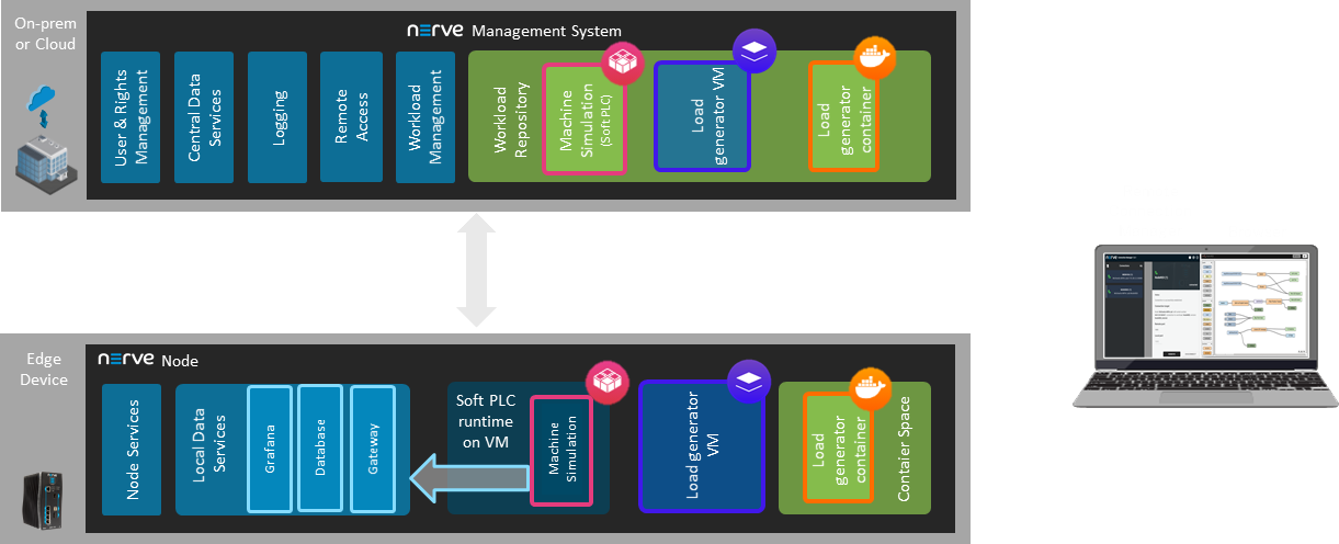
The machine simulation, Grafana and Gateway configuration UI are accessed on the Nerve Device directly using the remote access feature of the Nerve cloud management platform called the Nerve Management System. In Nerve, applications managed by customers are called workloads. The Management System is a Software-as a Service hosted in Microsoft Azure. The device is located in TTTech Industrial’s Nerve labs.
Initial setup
The Nerve Management System is set up so that the tutorial can be started straightaway. The necessary applications have already been configured and the remote connections are set up. The evaluation system does not limit experimentation to the extent of this tutorial. It is possible to create, deploy and test new workloads. However, the cloud instance of the Data Services and user management are not enabled in the standard evaluation system. Also note that this tutorial is designed to be done with Nerve Devices running an ACRN hypervisor, meaning that snapshots of virtual machines are not available since they rely on the KVM hypervisor. Contact sales@tttech-industrial.com for information on how to obtain the full version.
To explore the Nerve system even further, refer to the user guide.
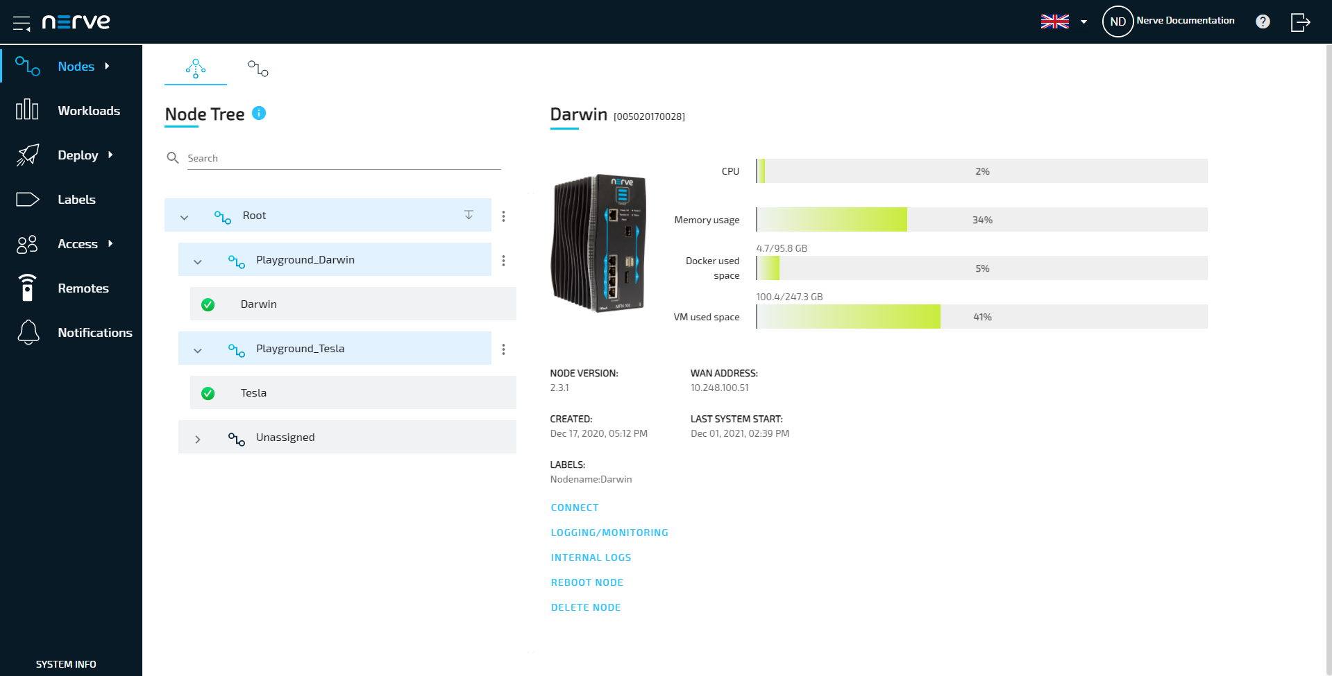
Viewing nodes in the node tree
The node tree is the first visible page of the Management System after logging in. It presents a means of organization for nodes that are connected to the Management System. Nodes are embedded into elements of the node tree.
- Log in to the Management System with your credentials.
-
Look for your node in the node tree. It is embedded in its own tree element.
Note
The node and the tree element are named after a scientist. The name has been sent in an email.
Be aware that other users may access the same evaluation system. Make sure to use the designated node that was mentioned in the instruction emails.
Step 1: Deploying the machine simulation
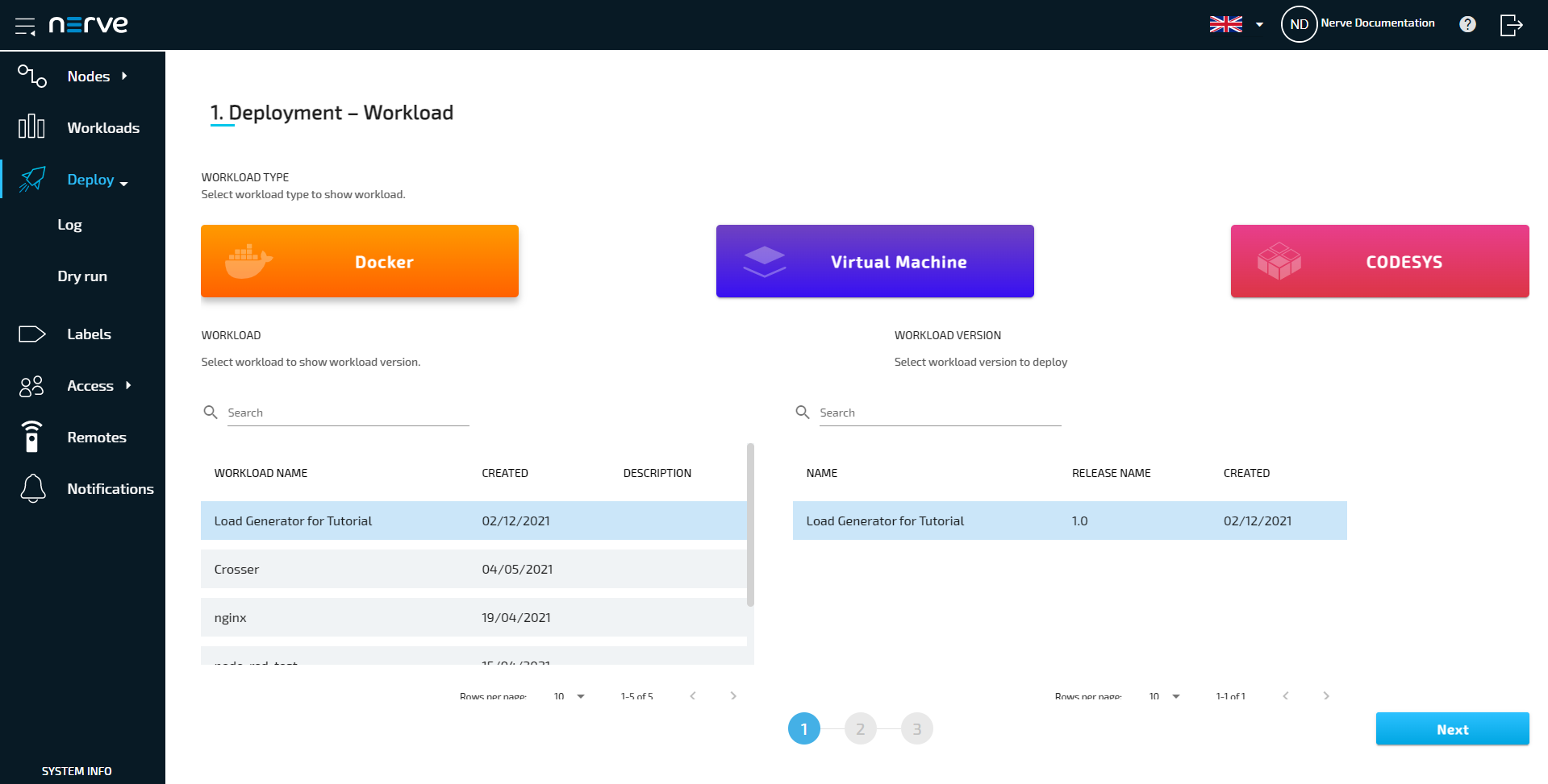
Deployment is the process of downloading workloads to Nerve Devices through the Nerve Management System. With Nerve you can deploy and manage Docker containers, virtual machines and CODESYS applications. The instructions below show how to deploy the machine simulation as a CODESYS workload.
- Log in to the Management System.
-
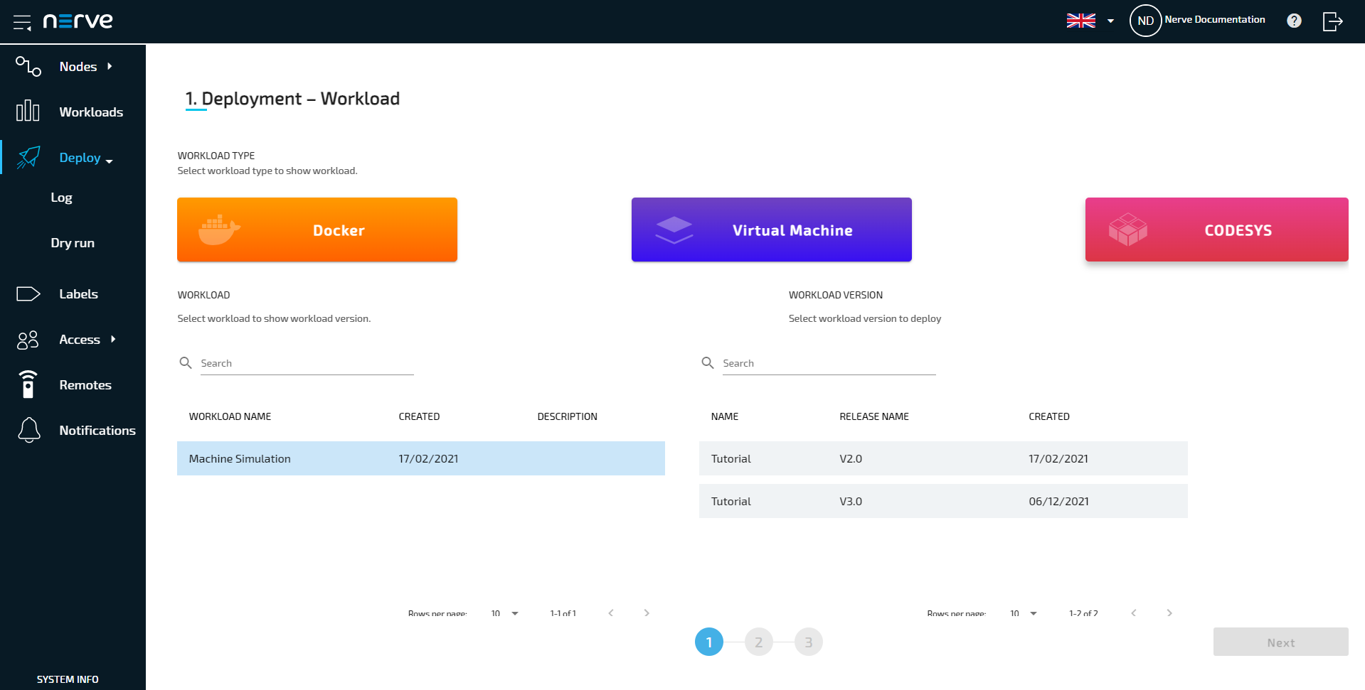
Select Deploy in the navigation on the left.
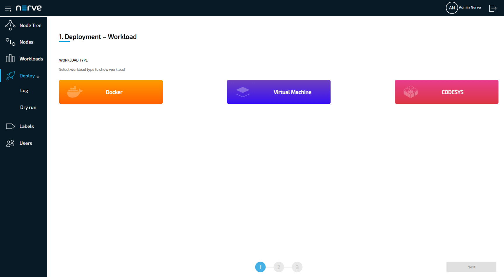
-
Select the red CODESYS tab. A list of CODESYS workloads will appear below.
-
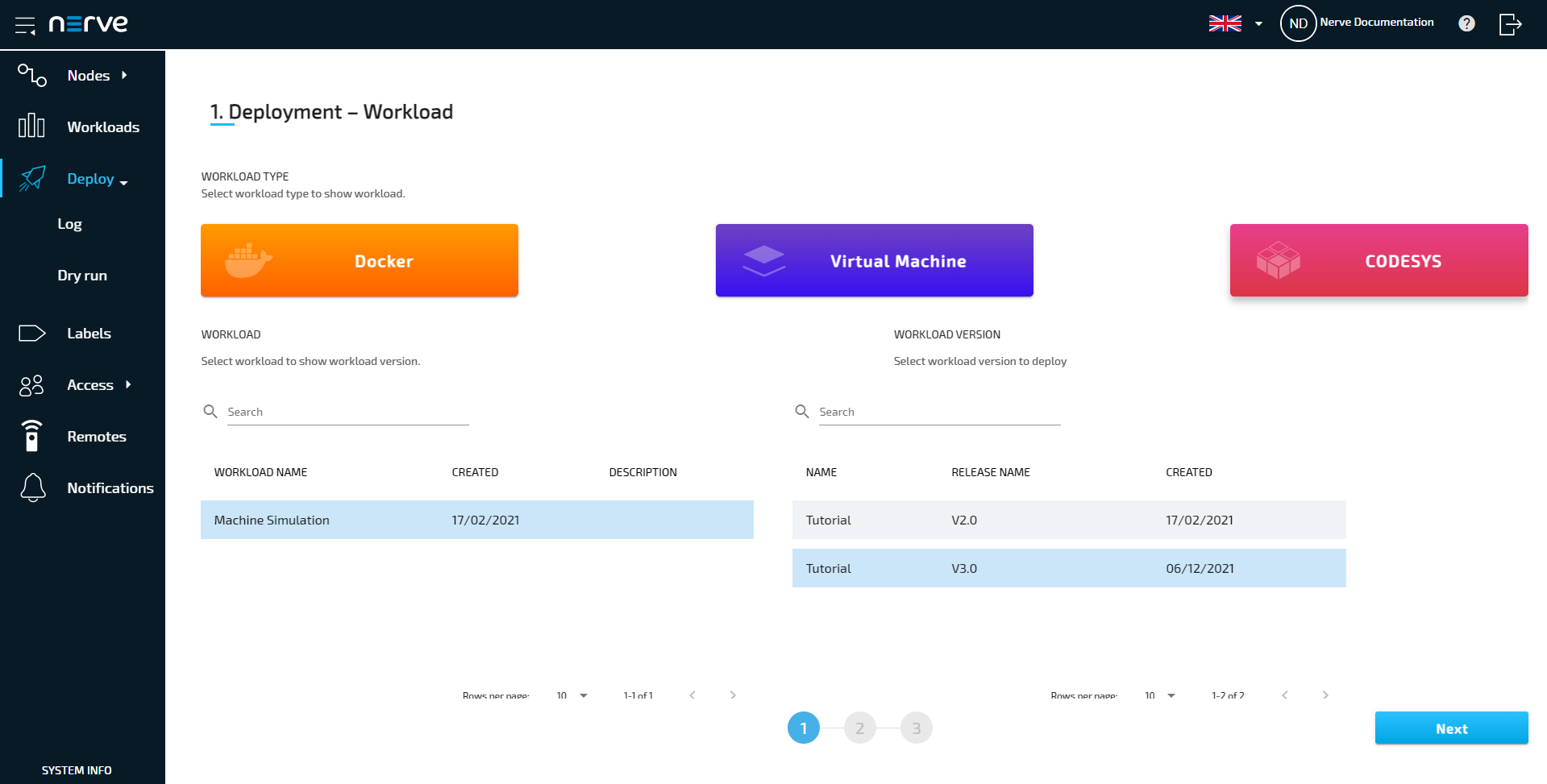
Select Machine Simulation in the list of workloads. A list of versions of this workload will appear to the right.
-
Select V3.0 on the right.
-
Select Next in the lower-right corner.
-
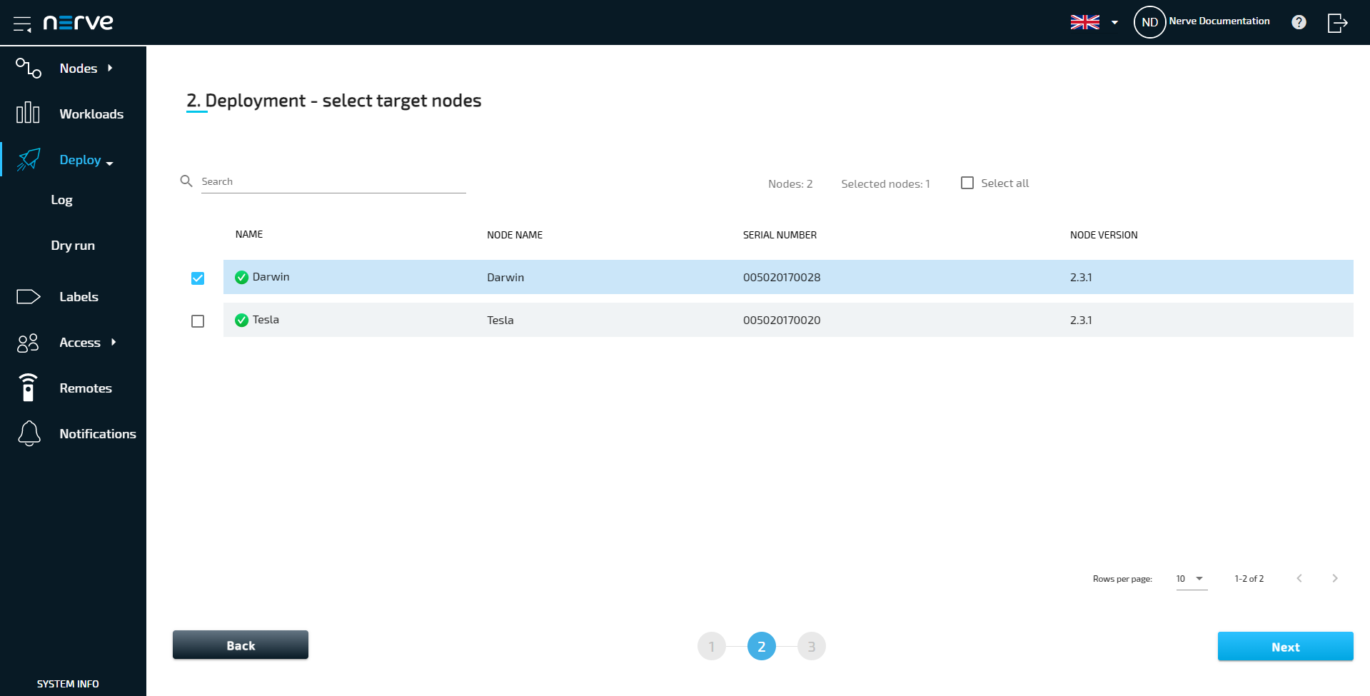
Tick the checkbox next to your node.
-
Select Next in the lower-right corner.
-
Select Deploy to execute the deployment.
Optional: Enter a Deploy name above the Summary of the workload to make this deployment easy to identify. A timestamp is filled in automatically.
The deployment should now be visible at the top of the deployment log. Click the log entry of the deployment to see a more detailed view.
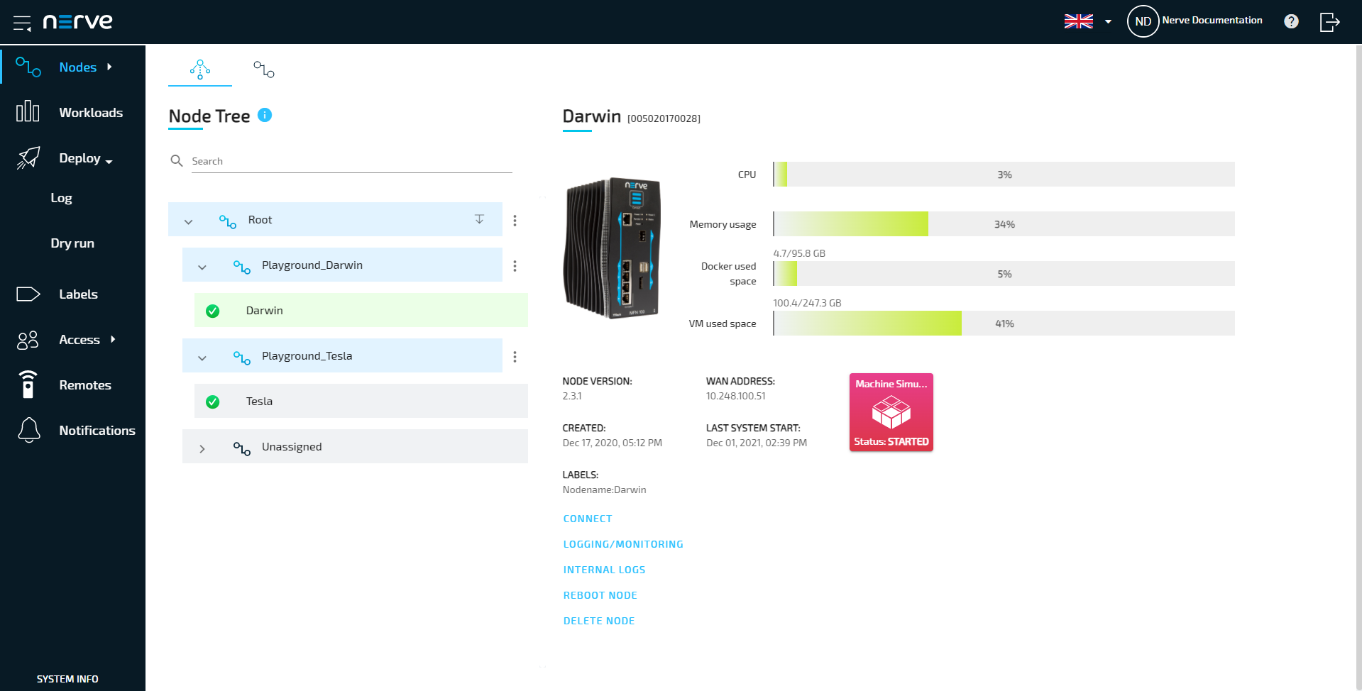
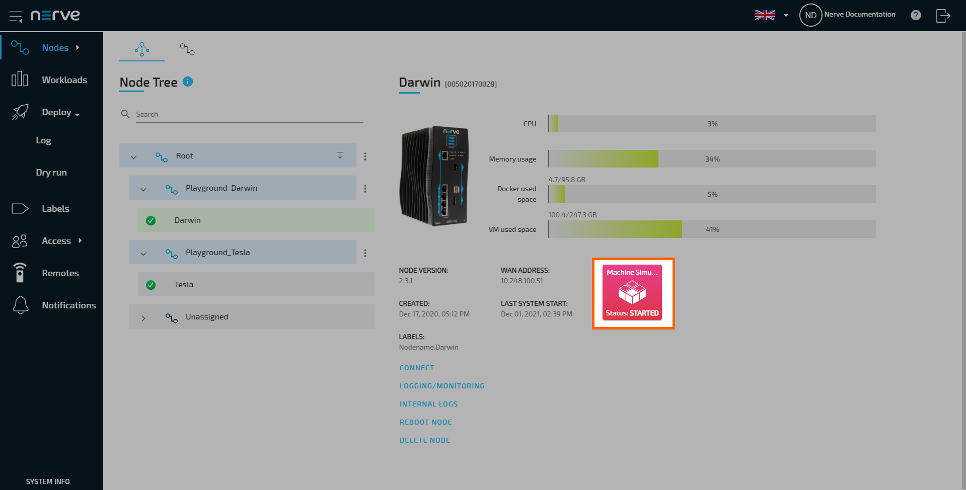
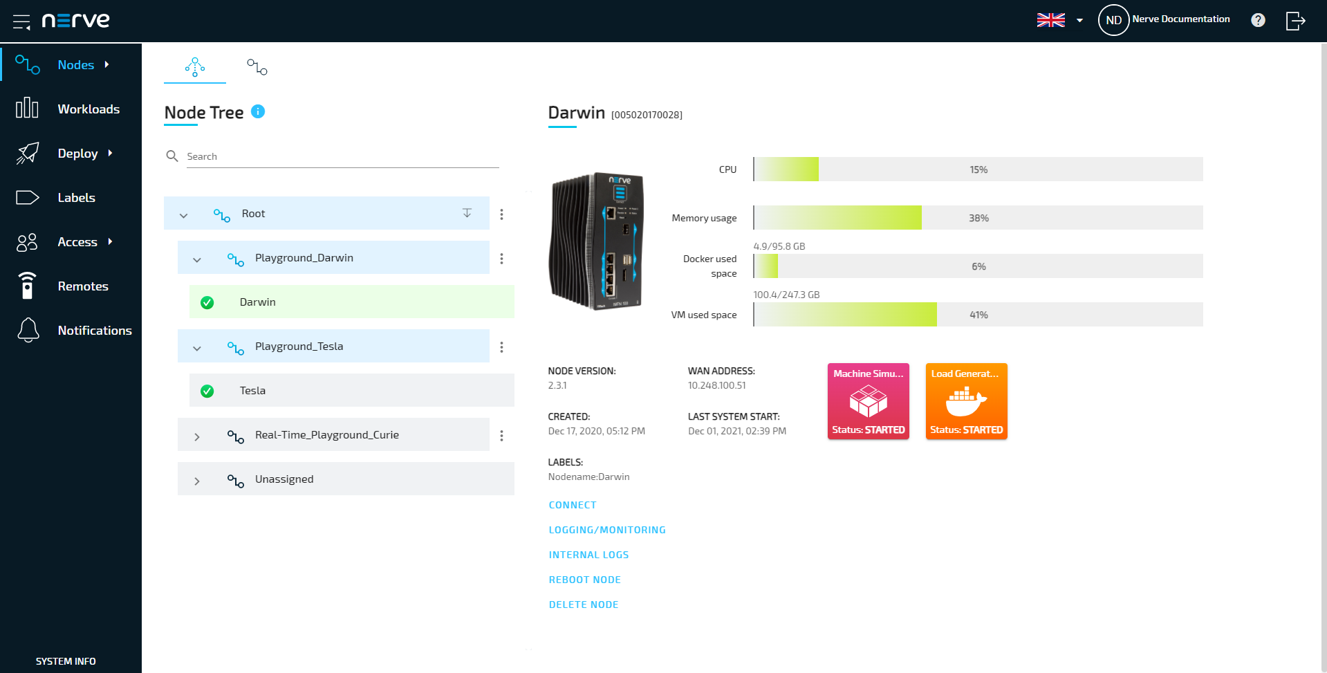
To confirm if the workload has been deployed successfully, select Nodes in the navigation on the left. Select your node in the node tree and confirm if a CODESYS workload tile is showing underneath the bar graph. The workload should show the status STARTED.
Note
It can take a number of seconds until the status of a workload switches from IDLE to STARTED after deployment.
Step 2: Connecting to the machine simulation through remote access
To access the machine simulation, it is required to create a connection between the computer used for this tutorial and the Management System, and from the Management System to the webserver of the machine simulation on the Nerve Device. This is done through the remote access feature, specifically through the use of remote tunnels. The remote tunnel connection has already been configured in the Management System and is ready for use. The image below illustrates the remote access feature, showing a connection to the deployed machine simulation on the Nerve Device.
The machine simulation is accessible at port 8080 on the Nerve Device through a web user interface. The pre-configured remote tunnel will use this port and port 8080 on the local computer to create a connection between the computer and the Nerve Device to access the machine simulation.
Before continuing, install the Nerve Connection Manager that was part of the delivery, as it is required for using remote tunnels.
Note
Local admin rights might be required to successfully install the Nerve Connection Manager.
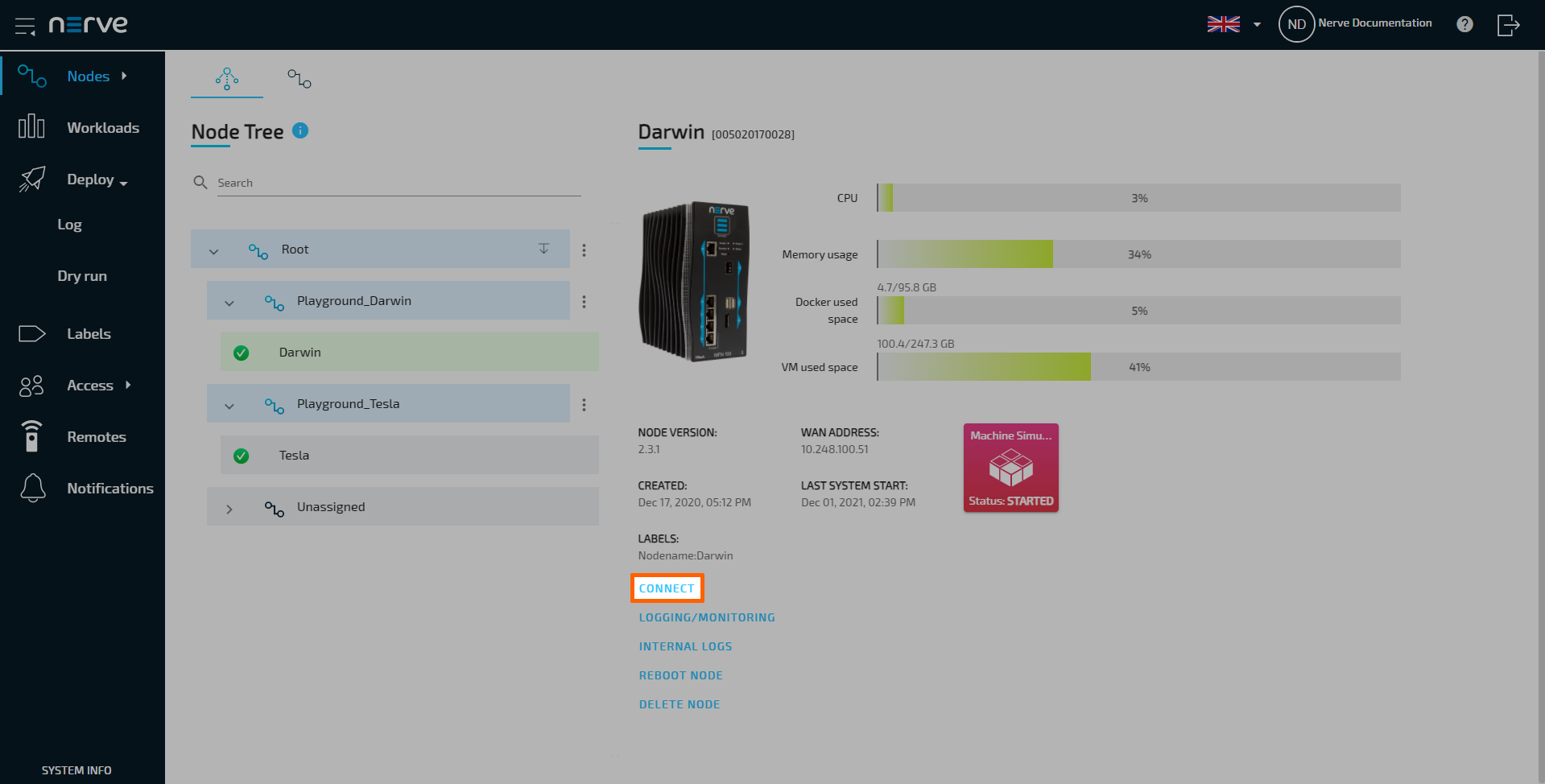
- Select Nodes in the navigation on the left.
- Select your node in the node tree.
-
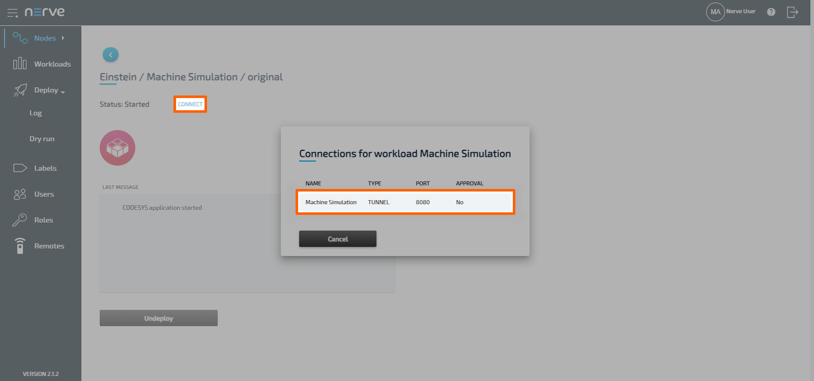
Select the Machine Simulation CODESYS workload.
-
Select CONNECT next to the workload status. Available connections will appear in a window.
-
Select the Machine Simulation remote tunnel from the list.
-
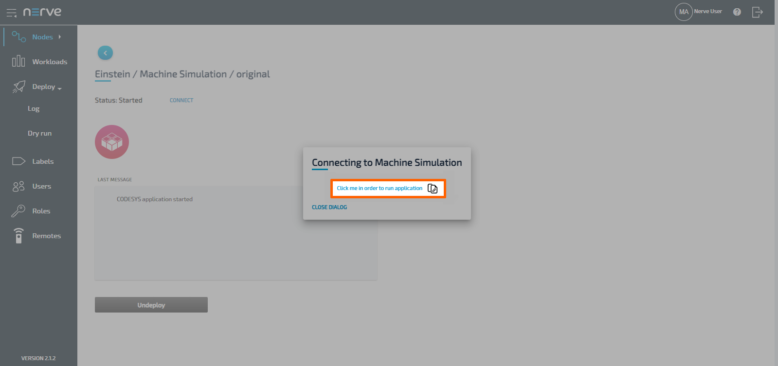
Select link in the new window.
-
If the Nerve Connection Manager installed correctly, confirm the browser message that the Nerve Connection Manager shall be opened.
Depending on the browser that is used, this message will differ. The Nerve Connection Manager will start automatically once the message is confirmed.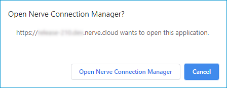
Note
If the Nerve Connection Manager does not start automatically, refer to Using a remote tunnel to a node or external device in the user guide.
The remote tunnel will be established once the Nerve Connection Manager starts and the remote connection will turn green in the Nerve Connection Manager. The remote tunnel is now ready to be used.
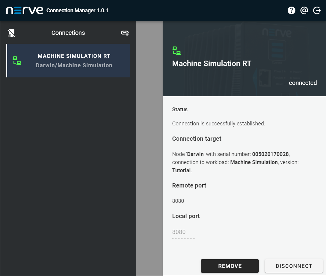
Open a new browser tab and enter localhost:8080 to open the machine simulation dashboard. The dashboard has two elements pertaining to jitter values, Task Jitter and Task Monitor.

The Task Jitter is a visual presentation of the jitter values. The green line shows the value of jitter in microseconds over time, either positive or negative, while the red lines show the highest recorded positive and negative jitter values.
At the bottom of the machine simulation interface, the jitter values can be observed in numerical form in the Task Monitor element. Refer to the explanation of each value below:
| Item | description |
|---|---|
| Jitter [us] | This is the currently recorded jitter value. |
| Jitter Neg [us] | This value shows the highest value recorded of how much earlier the task occured compared to the desired cycle. Example: -25 means that the task occurred 25 µs earlier as planned. |
| Jitter Pos [us] | This value shows the highest value recorded of how much later the task occured compared to the desired cycle. Example: 107 means that the task occurred 107 µs later than planned. |
| Delta [us] | This is the currently recorded cycle time in microseconds. The target is 1000 µs, i.e 1 ms. |
| Delta Min [us] | This is the lowest recorded cycle time in microseconds. |
| Delta Max [us] | This is the highest recorded cycle time in microseconds. |
Step 3: Configuring the Gateway
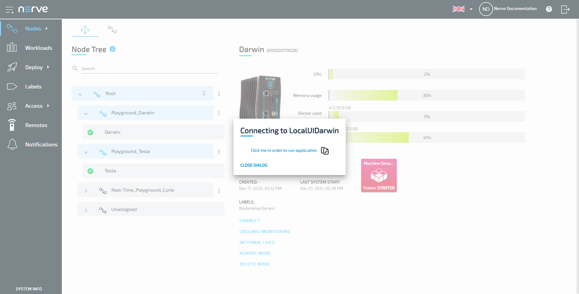
In order to configure the Gateway, we need to access the local user interface which runs on the Nerve Device itself. To do this, we need to connect to the user interface using the remote connection. The process is similar to the remote connection that was established to the machine simulation above. This time we are not establishing a connection to a workload but to the node itself.
- Select Nodes in the navigation on the left.
- Select your node in the node tree.
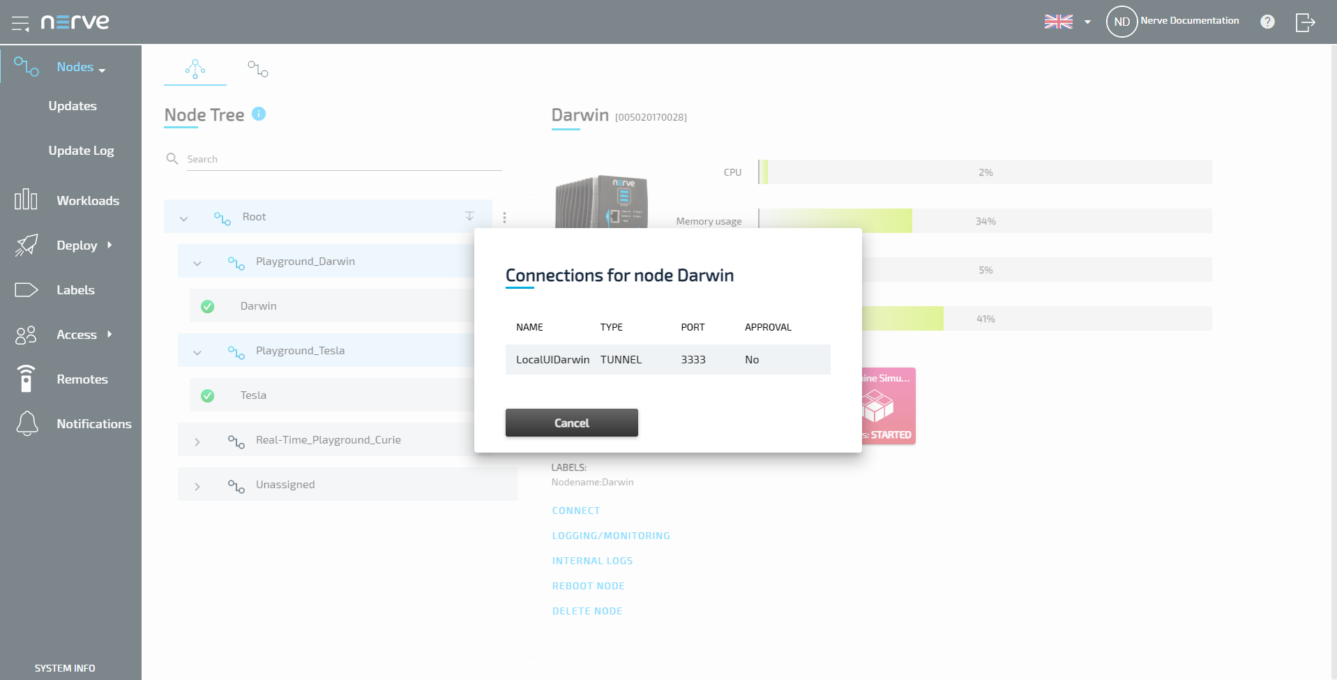
-
Select CONNECT in the list of commands underneath the device image. Available connections will appear in a window.
-
Select the LocalUI<scientistname> remote tunnel from the list.
-
Select link in the new window.
-
If the Nerve Connection Manager installed correctly, confirm the browser message that the Nerve Connection Manager shall be opened.
Depending on the browser that is used, this message will differ. The Nerve Connection Manager will start automatically once the message is confirmed.Note
If the Nerve Connection Manager does not start automatically, refer to Using a remote tunnel to a node or external device in the user guide.
The remote tunnel will be established once the Nerve Connection Manager starts and the remote connection will turn green in the Nerve Connection Manager. The remote tunnel is now ready to be used.
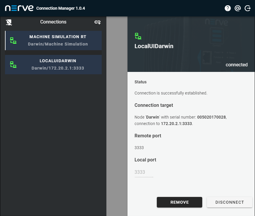
Open a new browser tab and enter localhost:3333 to open the Local UI of the Nerve Device. Log in to the Local UI. The login credentials to the Local UI have been sent by mail.

Applying the Gateway configuration and previewing data
The Gateway can be either configured by entering the configuration parameters into the graphical configuration tool or through importing a pre-written JSON configuration file. In this tutorial we will upload the configuration file that has been sent to you by email for the sake of simplicity.
The JSON configuration file contains:
- the configuration of the input variables which the Gateway should read from the PLC’s OPC UA server
- the output location – in this case the integrated Nerve database
- a defined connection between input and output
The configuration file also tells the Gateway to create a table named CodesysRealTimeData in the integrated Nerve database.
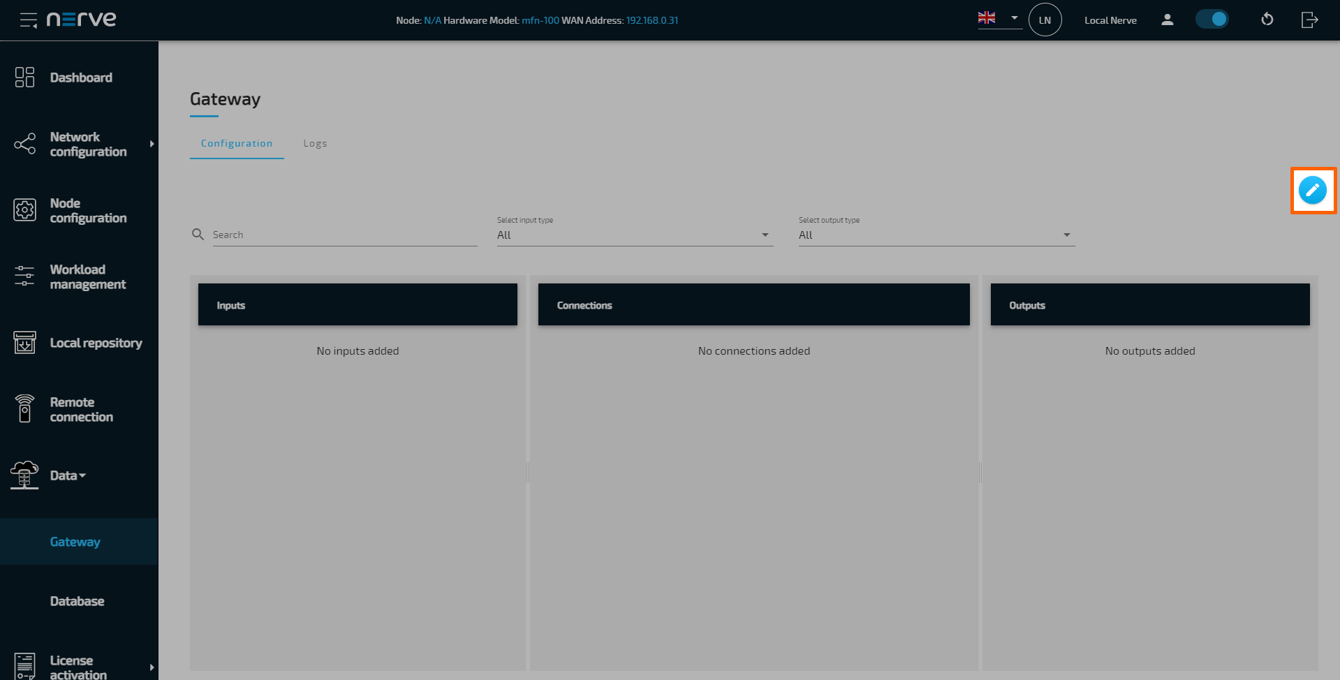
- In the Local UI, select the arrow next to Data to expand the Data Services sub menus in the navigation on the left.
- Select Gateway.
-
Select the Edit configuration icon on the right to enter editing mode.
-
Select the Import button.
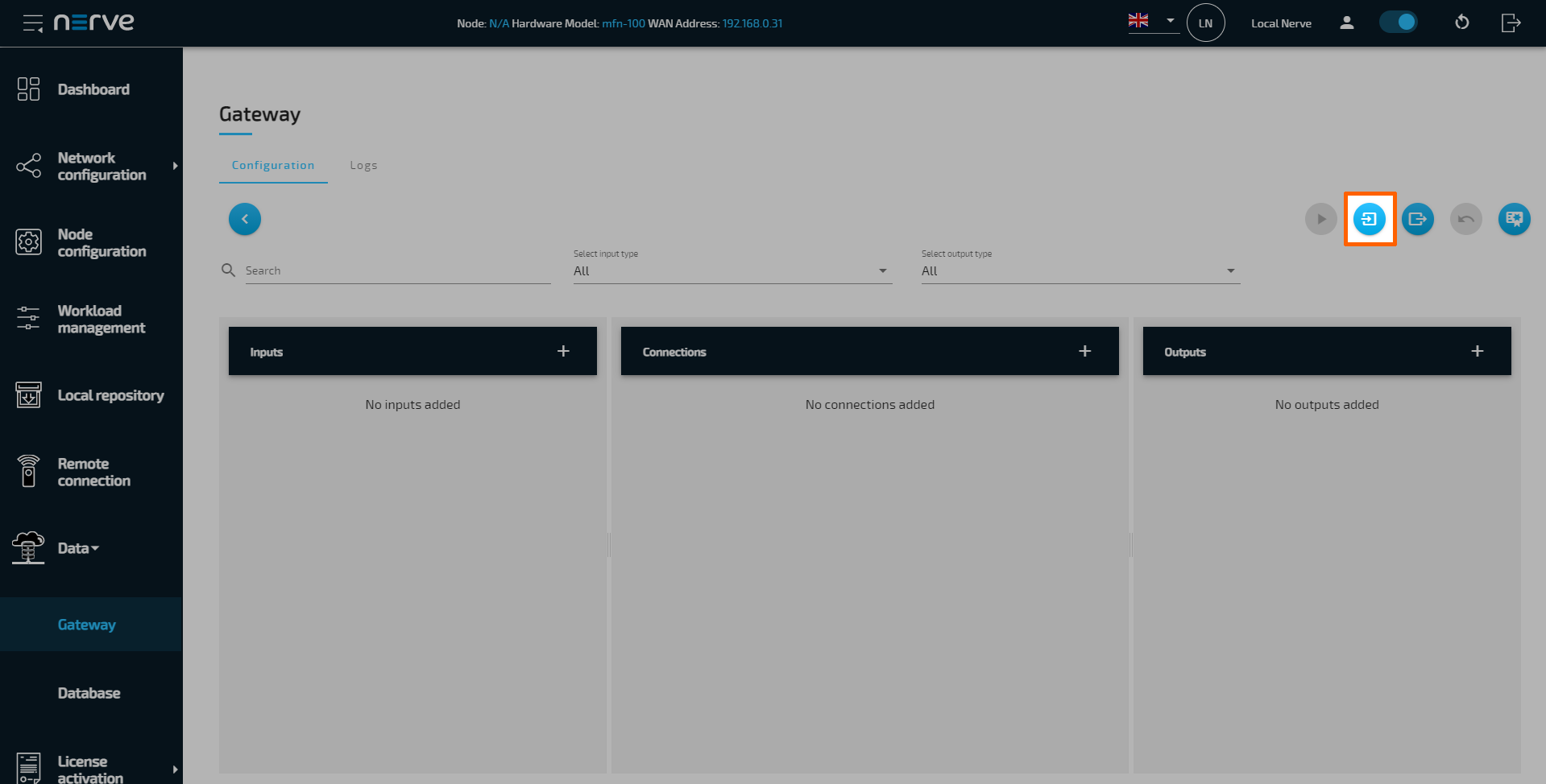
-
Import the Gateway configuration file that has been sent by mail.
-
Select the Deploy button. A success message pops up in the upper-right corner.
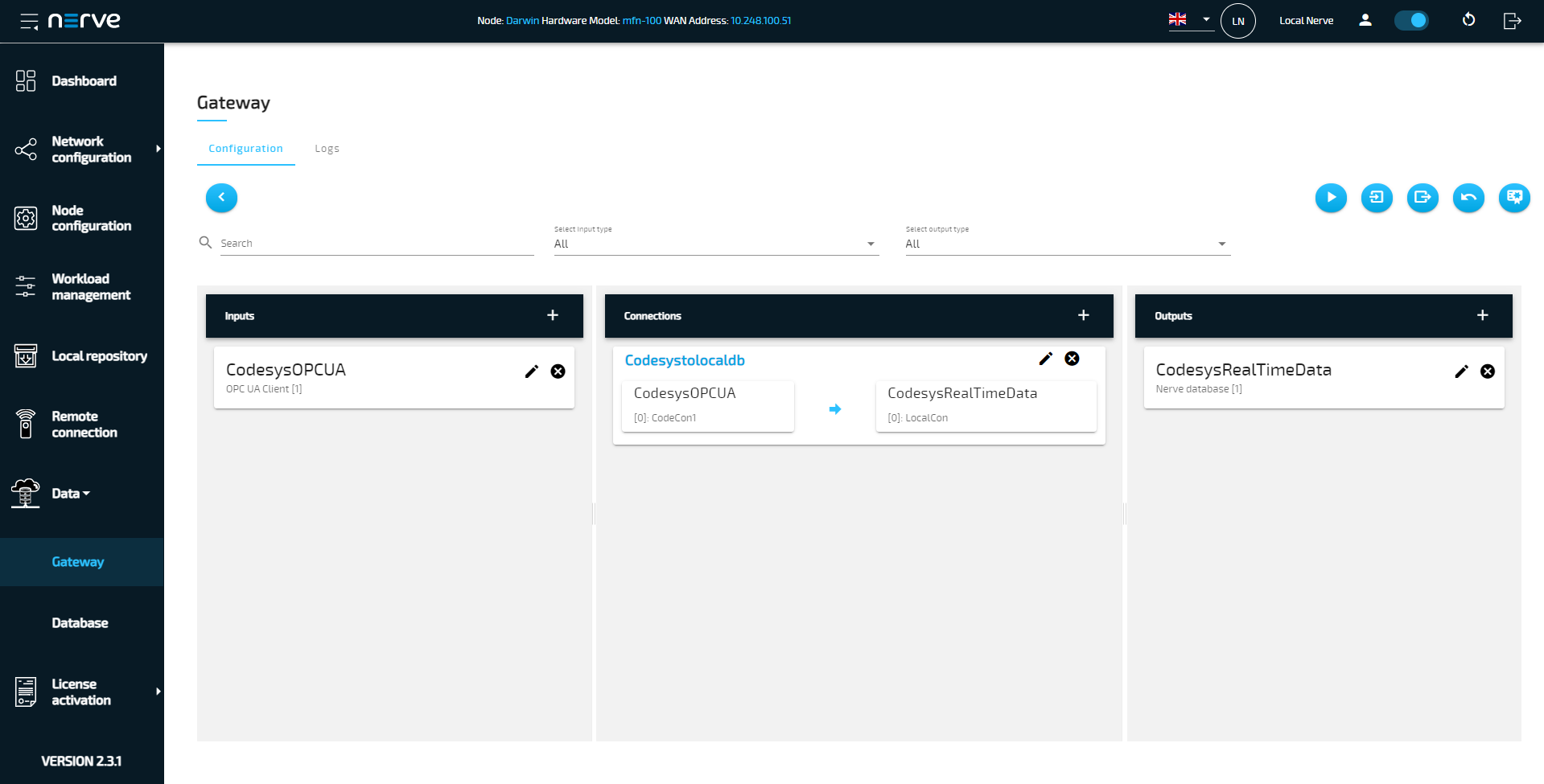
The configuration is now deployed. The graphical configuration tool now reflects the contents of the JSON file. Exit editing mode by selecting the arrow on the left. Details of each input and output can be opened by selecting the magnifying glass symbol next to each input and output.
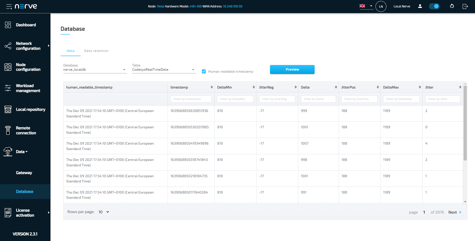
The jitter values that are collected by the Data Services can be previewed in the integrated database viewer. Select Data in the navigation on the left and select Database from the sub menu. Select nervedb_local from the drop-down menu labeled Database. Then select CodesysRealTimeData from the drop-down menu labeled Table.
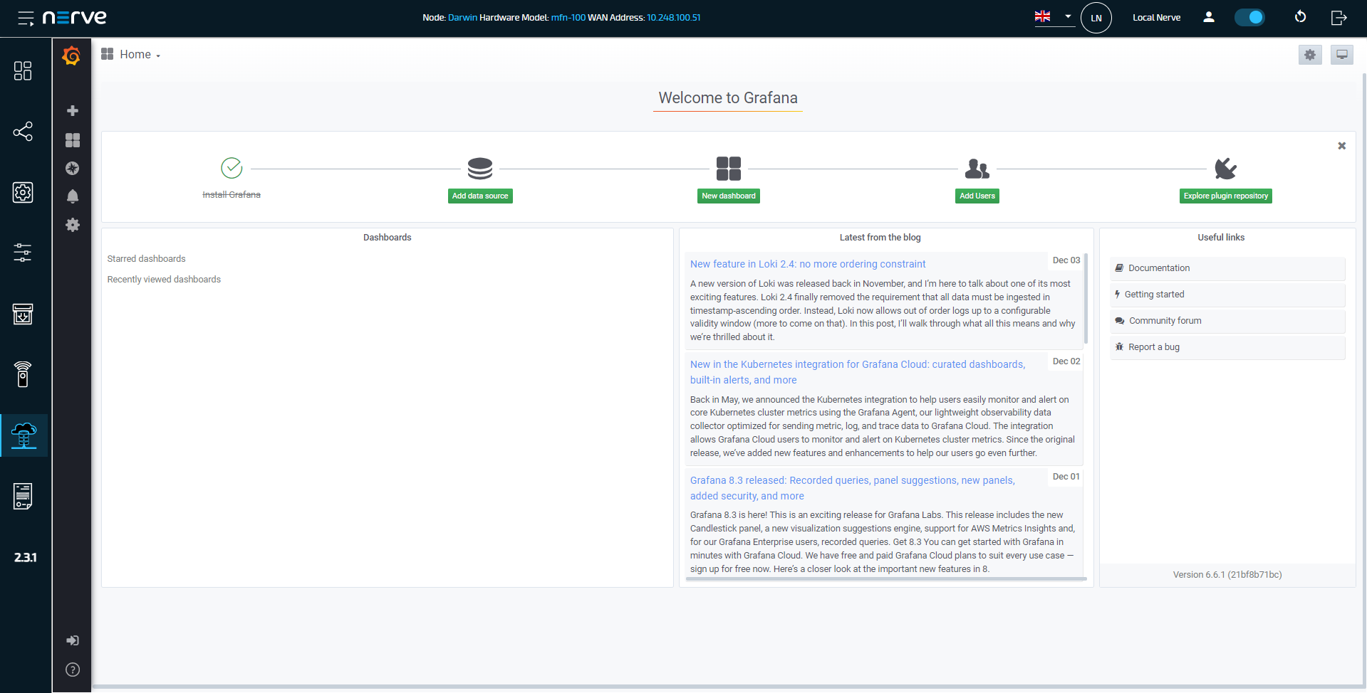
Step 4: Viewing jitter data in Grafana
After the deployment of the machine simulation and the configuration of the Gateway, jitter data is being collected. To view jitter data in Grafana, a dashboard needs to be created. For the sake of simplicity, we configured the dashboard beforehand. This file has been sent as part of the delivery. The instructions below cover how to import the dashboard.
- Select Data in the navigation on the left.
-
Select Home in the Grafana window.
-
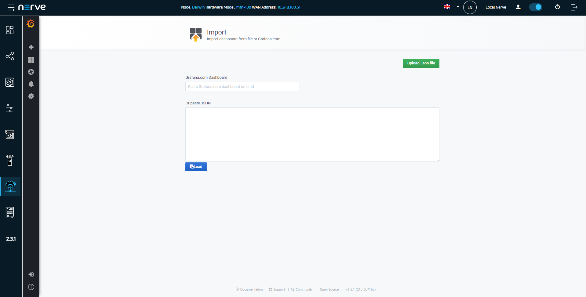
Select Import dashboard.
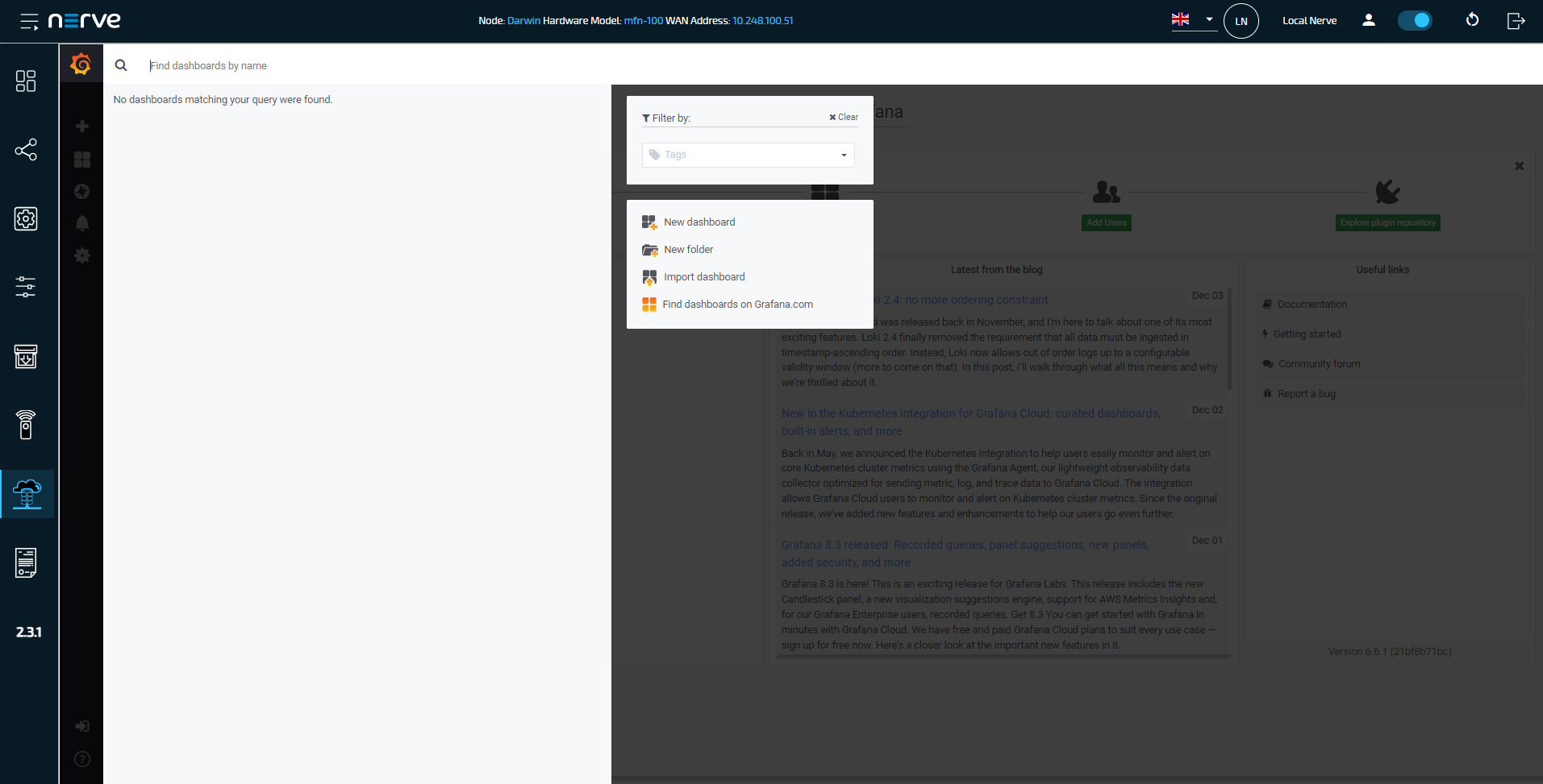
-
Select Upload .json file in the upper-right.
-
Select the jitter dashboard JSON file that was part of the delivery.
- Select Open.
-
Select the only available item from the data source selector drop-down menu. The data source corresponds to the serial number of the node.
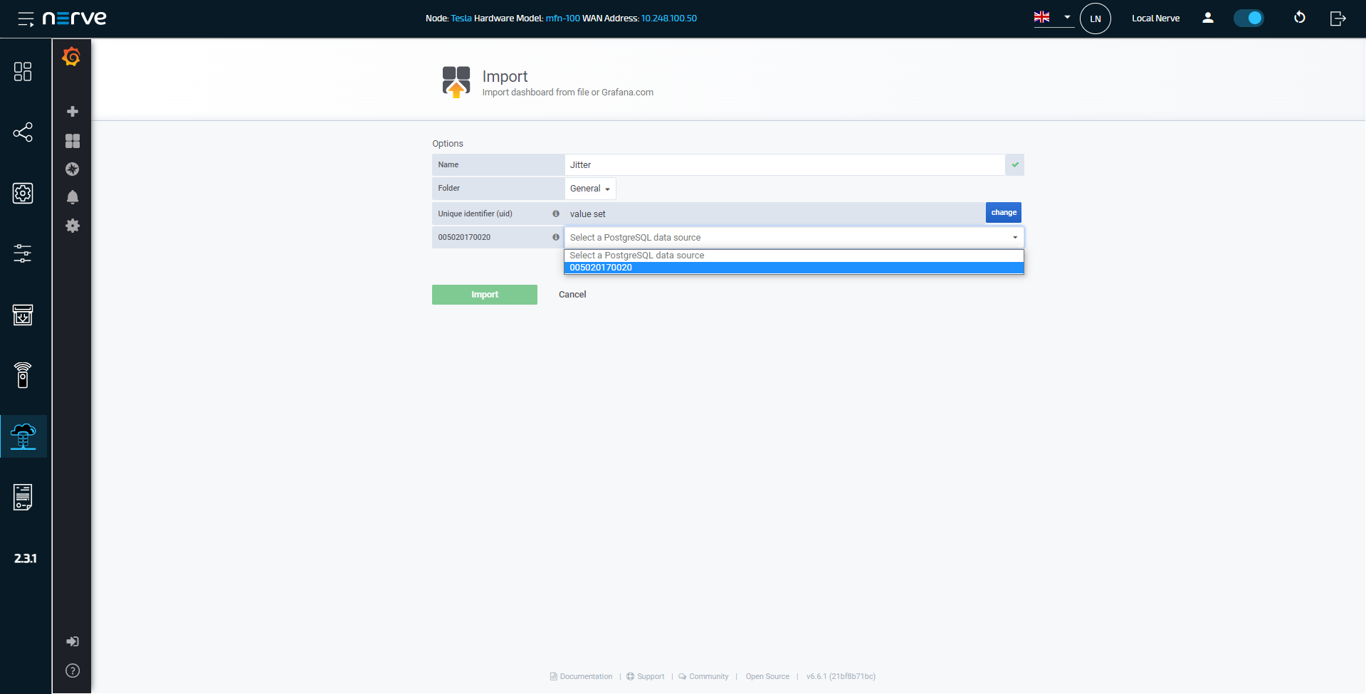
-
Select Import.
The Jitter dashboard is now created, showing two graphs, Jitter and time between task execution.
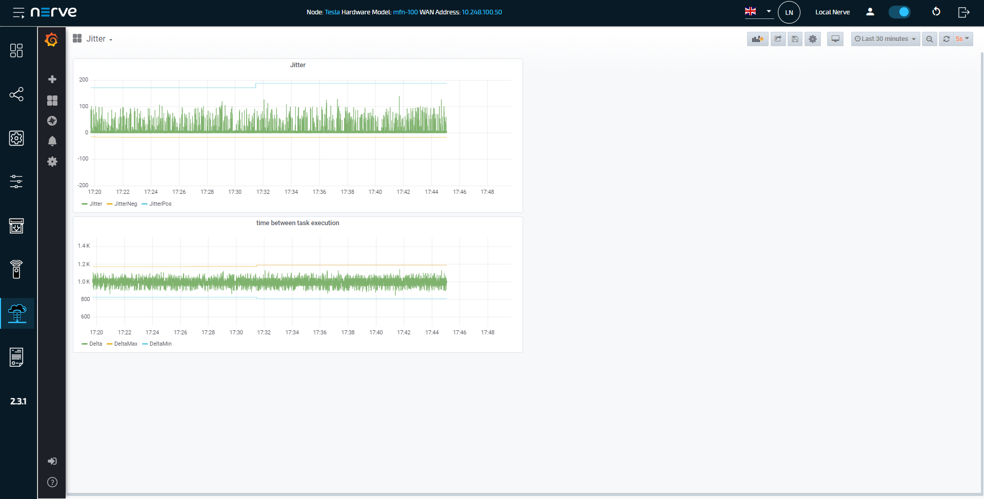
Similar to the machine simulation, the upper graph labeled Jitter shows the jitter value over time in microseconds (Jitter), the highest recorded positive jitter value (JitterPos) and the highest recorded negative jitter value (JitterNeg).
The lower graph labeled time between task execution shows the recorded cycle time values (Delta), the highest recorded cycle time (DeltaMax) and the lowest recorded cycle time (DeltaMin).
Step 5: Deploying the load generator workloads
In this step, we will deploy the aforementioned load generator workloads — a Docker container and a virtual machine. The instructions below will walk you through the deployment process for the Docker workload. Please repeat the process for the Virtual Machine workload.
-
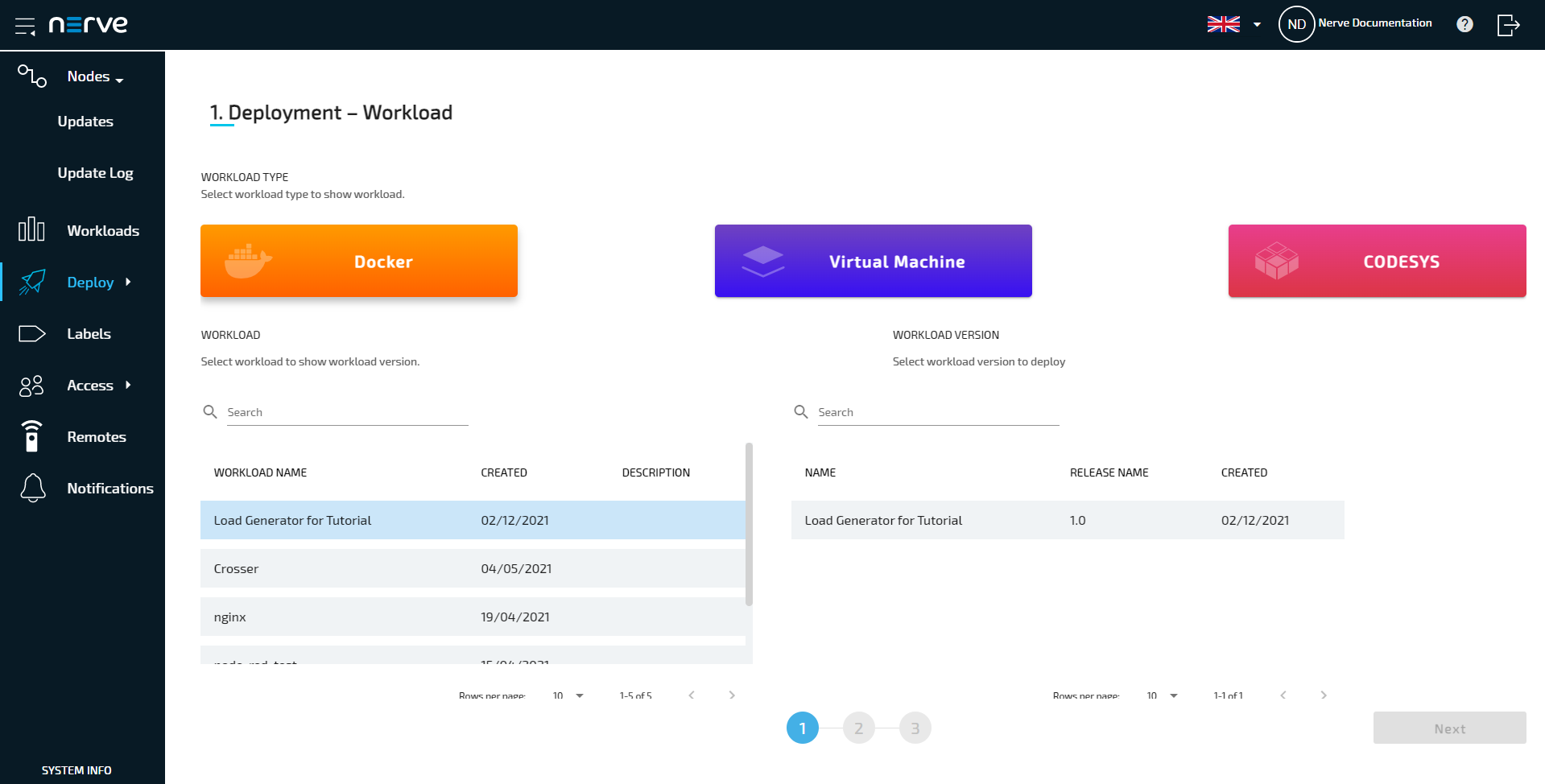
In the Management System, select Deploy in the navigation on the left.

-
Select the orange Docker tab. A list of Docker workloads will appear below.
-
Select the Load Generator for Tutorial workload from the list. A list of versions of this workload will appear to the right.
-
Select the latest version of the workload on the right.
-
Select Next in the lower-right corner.
-
Tick the checkbox next to your node.
-
Select Next in the lower-right corner.
-
Select Deploy to execute the deployment.
Optional: Enter a Deploy name above the Summary of the workload to make this deployment easy to identify. A timestamp is filled in automatically.
The deployment should now be visible at the top of the deployment log. Click the log entry of the deployment to see a more detailed view.
To confirm if the workload has been deployed successfully, select Nodes in the navigation on the left. Select your node in the node tree and confirm if a Docker workload tile is showing underneath the bar graph. The workload should show the status STARTED.
Note
It can take a number of seconds until the status of a workload switches from IDLE to STARTED after deployment.
To deploy the load generator VM, please repeat the steps above deploy the Virtual Machine workload. In step 2, select the blue Virtual Machine tab and pick the Load Generator on Alpine workload in its latest version. The remaining steps are identical.
Experiments and conclusion
What is jitter? Jitter is the deviation from the defined cycle time, and occurs when a task is performed earlier or later than planned. Take a look at the image below:
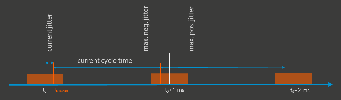
Starting from t0, tasks are targeted to occur every 1 ms. The planned task starts are symbolized by white lines in the image above. The actual task times, starting with tcycle start, are marked by orange lines and occur before or after the planned times. The difference between the planned and defined times is called jitter. Jitter values can therefore have positive and negative values, depending on when the cycle actually starts and finishes. Jitter values are negative if the cycle finishes before the planned time. Positive values occur when the cycle finishes later. In other words, this can be compared to a train schedule. If the train is too early or too late, jitter occurs.
The Nerve system guarantees a certain maximum jitter range to ensure real-time performance using the ACRN hypervisor, even when the system load is high. Now that the load generator workloads are deployed and operating, access the jitter dashboard in Grafana again to evaluate the difference in jitter data. Real-time performance should still be given. However, note that the load generator Docker container stops itself after 60 seconds. To have it generate system load again, start the Docker container again manually from the workload control screen in the node tree. To reach the workload control area, select the workload in the node details view in the node tree.